Programming Insight: Notes, Advice, and Evaluation Criteria for Python Programs
E N D
Presentation Transcript
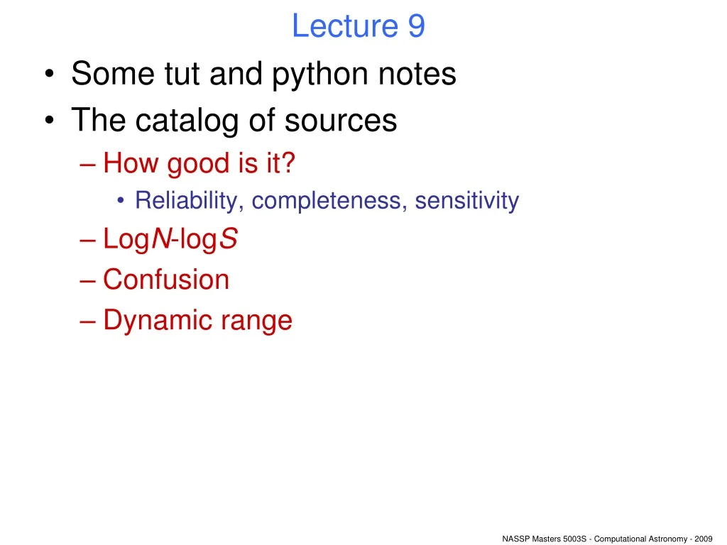
Lecture 9 • Some tut and python notes • The catalog of sources • How good is it? • Reliability, completeness, sensitivity • LogN-logS • Confusion • Dynamic range
Insight into Tut marking • Questions and proofs are marked in a standard fashion. Programs are more difficult. • My criteria for programs: • Does it run? • Is the algorithm correct? • Is it free from evil practices? • Are all the requirements addressed? • I give these four equal weight, and try to judge them separately. • PLUS one can earn extra marks by conspicuous use of some good programming habit.
Some remarks and advice about python programming. • The way to attack a problem is to attempt to break it into pieces and solve the pieces individually. • “If you don’t understand how to solve a problem, do any part of it you do understand, then look at the whole again.” (R Heinlein). • Programming is one of the few activities in which procrastination (putting unpleasant things off for later) can be a good thing.
Procrastination example • Tut 2, the MC: • It should be clear that you have to do something a million times. It may not be clear to you exactly what. So write a loop over the million times, and shove all the rest into a function: • A little more thought tells you that the function must return a chi squared value. So change to: • Worry about the function later! numIter = 1000000 for i in range(numIter): doSomething() numIter = 1000000 chi2Vals = [] for i in range(numIter): chi2Vals.append(calcChi2())
Remarks and advice continued. • The first most important thing your code should do is run, and the second is that it must work correctly. • If these criteria are not met, it is pointless to worry about “saving memory/time/characters.”
Remarks and advice continued • The pass statement makes a useful placeholder if your code is incomplete but you want to see if it runs. Eg • The raise statement is a useful way to stop the program if there is an error. Eg • Don’t forget that 2-d numpy arrays are in row-column order, not x-y. Ie, shape[0] is the number of rows, hence the size of the matrix in the Y direction, not the X. def calcChi2(): pass if calcChi2()<=0.0: raise ‘nonPosChi2’
Remarks and advice continued • Converting intfloatint again (as some of you did in tut 1) falls into the ugly category of evility. As such, I’ll deduct marks for it. • I won’t penalize the following, but I think they are bad ideas: • Use of raw_input rather than sys.argv. • The reason is you may want to run your python programs from within a script. You can’t do that if the program blocks for input. • Omitting the #!/usr/bin/env python. • If you don’t have this, and forget and attempt to run your program as a stand-alone, you will get some weird results! (Among other reasons, because import is also a unix command.)
How to analyse the source catalog. • Things we want to know: • Reliability: • The number (or fraction) of false positives. • Completeness: • The fraction of real sources we are finding. People say things such as “the survey is essentially complete at a flux greater than so-and-so.” • Sensitivity: • Broadly speaking this is the flux at which we are only detecting 50% of the sources. • These are often not very exactly defined terms.
A source-detection Monte Carlo: • Things to note from this plot: • Fainter sources become more numerous… • …until a cutoff value of S. • Measured ^S is scattered about true S. • The ^S distribution is biased at low S.
The logN–logS plot. • In a ‘Euclidean universe’, • Therefore • But Olbers’ paradox says there must be a cutoff. • This is observed in several actual surveys. => large-scale structure. Input fluxes
Eddington bias • Happens because measured flux ^S is random – it is scattered about the true value. • The result is a ‘blurring’ of the ‘true’ logN-logS. • Because usually n(S) has a negative slope, this blurring inflates the number of sources. Red: ‘measurable’ fluxes
How does our catalog shape up? • The really interesting things in the logN-logS curve always seem to be happening just at our sensitivity limit. 2 things to do: • Persuade ESA/NASA etc to spend $$$$ on a bigger and better telescope; • What do you mean, “don’t be ridiculous?” • Ok then, let’s lower the Pcutoff. • But… Blue: ‘true’ detections
…Don’t forget the falsies. • Next episode: Confusion, dynamic range. Cyan: false detections.
Confusion A NICMOS exposure towards the galactic centre. Credit: Spitzer Science Centre/STScI An all-instrument mosaic of XMM EPIC cameras. A rich stellar cluster.
A 1D simulation. • Start with a distribution of sources. Euclidean model gives: • Each source has some random structure. • They also vary in width. n(S) αS-5/2 (Actually I used a lower power to make the plots look better.)
A 1D simulation. • Add in instrumental broadening. • Now every source looks much the same. • ‘Unresolved sources’. • Most sources in eg optical, radio, x-ray images are unresolved.
A 1D simulation. • And finally, add noise. (Remember, it can happen the other way around – first noise then broadening.) • Sensitivity here is limited by noise. • Suppose we push the noise right down, by observing longer, or with a more sensitive instrument…?
Confusion • …Eventually the sensitivity becomes confusion-limited. • At each point in the sky, the nett flux is a sum of contributions from >1 source. • Brightest contributor named the confused source; its flux and position are distorted. • All fainter are not directly observable. • But, can get statistical info on n(S) from noise distribution.
Two possible remedies: • Subtract sources, starting with the brightest. • Eg the CLEAN algorithm in radio interferometry. • Eg 2: sExtractor. Brightest subtracted
The other possible remedy: • Try to reduce the instrumental broadening.
Higher resolution • Methods: • Via hardware: wider aperture – higher resolution. • Or software: deconvolution (eg Maximum Entropy). • The fundamental limit comes from the widths of the objects themselves – ‘natural confusion.’
Eg the Hubble Deep Field. Credit STScI
Example of bright source subtraction: Planet 1 Planet 2 Credit: Gemini Observatory/AURA
Another example: hot gas around Cen B Raw Smoothed Bright sources subtracted Dummy Schroeder, Mamon and Stewart – in preparation.
Dynamic range • The problem with this is that the subtraction may not be perfect. • Imperfect measurement of source position or flux. • Calibration errors (interferometry). • Imperfect knowledge of the source profile (XMM). • Ratio of brightest source to remaining artifacts called the dynamic range. Imperfect subtraction of the PSF in a MERLIN image. Best dynamic range only 104 (=40 dB).
