Graph Algorithm
Graph Algorithm. http://net.pku.edu.cn/~course/cs202/2014 Hongfei Yan School of EECS, Peking University 5/21/2014. Contents. 01 Programming: A General Overview (20-65) 02 Algorithm Analysis (70-89) 03 Lists, Stacks, and Queues (96-135) 04 Trees (140-200) 05 Hashing (212-255)

Graph Algorithm
E N D
Presentation Transcript
Graph Algorithm http://net.pku.edu.cn/~course/cs202/2014 Hongfei Yan School of EECS, Peking University 5/21/2014
Contents • 01 Programming: A General Overview (20-65) • 02 Algorithm Analysis (70-89) • 03 Lists, Stacks, and Queues (96-135) • 04 Trees (140-200) • 05 Hashing (212-255) • 06 Priority Queues (Heaps) (264-302) • 07 Sorting (310-360) • 08 The Disjoint Sets Class (370-393) • 09 Graph Algorithms (398-456) • 10 Algorithm Design Techniques (468-537)
Outline • Definitions • Topological Sort • Shortest-Path Algorithms • Network Flow Problems • Minimum Spanning Tree • Applications of Depth-First Search • Introduction to NP-Completeness
Definitions (1/4) • A graphG = (V, E) consists of a set of vertices, V, and a set of edges, E. • Each edge is a pair (v, w), where v, w ∈ V. Edges are sometimes referred to as arcs. • If the pair is ordered, then the graph is directed. • Directed graphs are sometimes referred to as digraphs. • Vertex w is adjacentto v if and only if (v, w) ∈ E. • In an undirected graph with edge (v, w), and hence (w, v), w is adjacent to v and v is adjacent to w. • Sometimes an edge has a third component, known as either a weightor a cost.
Definitions (2/4) • A pathin a graph is a sequence of vertices w1,w2,w3,...,wNsuch that (wi,wi+1) ∈ E for 1 ≤ i < N. • The lengthof such a path is the number of edges on the path, which is equal to N − 1. • If the graph contains an edge (v, v) from a vertex to itself, then the path v, v is sometimes referred to as a loop. • The graphs we will consider will generally be loopless. A simple pathis a path such that all vertices are distinct, except that the first and last could be the same.
Definitions (3/4) • A cyclein a directed graph is a path of length at least 1 such that w1 = wN; this cycle is simple if the path is simple. For undirected graphs, we require that the edges be distinct. • A directed graph is acyclicif it has no cycles. • A directed acyclic graph is sometimes referred to by its abbreviation, DAG.
Definitions (4/4) • An undirected graph is connectedif there is a path from every vertex to every other vertex. • A directed graph with this property is called strongly connected. • If a directed graph is not strongly connected, but the underlying graph (without direction to the arcs) is connected, then the graph is said to be weakly connected. • A complete graph is a graph in which there is an edge between every pair of vertices.
Airport system modeled by a graph • Each airport is a vertex, and two vertices are connected by an edge if there is a nonstop flight from the airports that are represented by the vertices. • The edge could have a weight, representing the time, distance, or cost of the flight. It is reasonable to assume that such a graph is directed, • since it might take longer or cost more (depending on local taxes, for example) to fly in different directions. • probably like to make sure that the airport system is strongly connected, so that it is always possible to fly from any airport to any other airport. • also like to quickly determine the best flight between any two airports. “Best” could mean the path with the fewest number of edges or could be taken with respect to one, or all, of the weight measures.
Traffic flow modeled by a graph • Each street intersection represents a vertex, and each street is an edge. • The edge costs could represent, among other things, a speed limit or a capacity (number of lanes). • ask for the shortest route or use this information to find the most likely location for bottlenecks.
9.1.1 Representation of Graphs • A directed graph, represents 7 vertices and 12 edges.
An adjacency matrix • use a two-dimensional array to represent a graph is known as an adjacency matrixrepresentation. • For each edge (u, v), set A[u][v] to true; otherwise the entry in the array is false. • If the edge has a weight associated with it, set A[u][v] equal to the weight and use either a very large or a very small weight as a sentinel to indicate nonexistent edges. • For instance, if we were looking for the cheapest airplane route, we could represent nonexistent flights with a cost of ∞. • If we were looking, for some strange reason, for the most expensive airplane route, we could use −∞ (or perhaps 0) to represent nonexistent edges.
Dense and sparse graph • An adjacency matrix is an appropriate representation if the graph is dense: |E| = Θ(|V|2). • In most of the applications that we shall see, this is not true. • E.g., any intersection is attached to roughly four streets, so if the graph is directed and all streets are two-way, then |E| ≈ 4|V|. • If there are 3,000 intersections, then we have a 3,000-vertex graph with 12,000 edge entries, which would require an array of size 9,000,000. • Most of these entries would contain zero.
Adjacency list • if the graph is sparse, a better solution is an adjacency list representation. • For each vertex, we keep a list of all adjacent vertices. • The space requirement is then O(|E| + |V|), which is linear in the size of the graph. • If the edges have weights, then this additional information is also stored in the adjacency lists. • A common requirement in graph algorithms is to find all vertices adjacent to some given vertex v
An adjacency list representation of a graph • to quickly obtain the list of adjacent vertices for any vertex, the two basic options are • to use a map in which the keys are vertices and the values are adjacency lists, • or to maintain each adjacency list as a data member of a Vertex class. • The first option is arguably simpler, but the second option can be faster, • because it avoids repeated lookups in the map.
if the vertex is a string • for instance, an airport name, or the name of a street intersection, • then a map can be used in which the key is the vertex name and the value is a Vertex (typically a pointer to a Vertex), • and each Vertex object keeps a list of (pointers to the) adjacent vertices and perhaps also the original string name.
Outline • Definitions • Topological Sort • Shortest-Path Algorithms • Network Flow Problems • Minimum Spanning Tree • Applications of Depth-First Search • Introduction to NP-Completeness
A topological sort • A topological sort is an ordering of vertices in a DAG, such that if there is a path from vito vj, then vjappears after viin the ordering. • The graph in Figure 9.3 represents the course prerequisite structure at a university. • A directed edge (v, w) indicates that course v must be completed before course w may be attempted. • A topological ordering of these courses is any course sequence that does not violate the prerequisite requirement.
Figure 9.3 An acyclic graph representing course prerequisite structure • a topological ordering is not possible if the graph has a cycle, • since for two vertices v and w on the cycle, v precedes w and w precedes v.
Figure 9.4 An acyclic graph • the ordering is not necessarily unique; any legal ordering will do. In the graph, v1, v2, v5, v4, v3, v7, v6 and v1, v2, v5, v4, v7, v3, v6 are both topological orderings.
A simple algorithm to find a topological ordering • find any vertex with no incoming edges. • then print this vertex, and remove it, along with its edges, from the graph. • apply this same strategy to the rest of the graph.
the indegree of a vertex v • The indegree of a vertex v as the number of edges (u, v). • compute the indegrees of all vertices in the graph. Assuming that the indegree for each vertex is stored, • and that the graph is read into an adjacency list, we can then apply the algorithm to generate a topological ordering.
implement the box, we can use either a stack or a queue • Because findNewVertexOfIndegreeZero is a simple sequential scan of the array of ver- tices, each call to it takes O(|V|) time. Since there are |V| such calls, the running time of the algorithm is O(|V|2). • remove this inefficiency by keeping all the (unassigned) vertices of indegree 0 in a special box. • The findNewVertexOfIndegreeZero function then returns (and removes) any vertex in the box. • When decrement the indegrees of the adjacent vertices, check each vertex and place it in the box if its indegree falls to 0.
To implement the box • use either a stack or a queue; we will use a queue. • First, the indegree is computed for every vertex. Then all vertices of indegree 0 are placed on an initially empty queue. • While the queue is not empty, a vertex v is removed, and all vertices adjacent to v have their indegrees decremented. • A vertex is put on the queue as soon as its indegree falls to 0. • The topological ordering then is the order in which the vertices dequeue.
Pseudocode to perform topological sort • The time to perform this algorithm is O(|E| + |V|) if adjacency lists are used.
Computing the indegrees • the cost of this computation is O(|E| + |V|) .
Outline • Definitions • Topological Sort • Shortest-Path Algorithms • Network Flow Problems • Minimum Spanning Tree • Applications of Depth-First Search • Introduction to NP-Completeness
Definitions • The input is a weighted graph: Associated with each edge (vi,vj) is a cost ci,jto traverse the edge. The cost of a path v1v2 . . . vNis This is referred to as the weighted path length. • The unweighted path length is merely the number of edges on the path, namely, N − 1.
Single-Source Shortest-Path Problem • Given as input a weighted graph, G = (V, E), and a distinguished vertex, s, find the shortest weighted path from s to every other vertex in G.
A directed graph G • the shortest weighted path from v1 to v6 has a cost of 6 and goes from v1 to v4 to v7 to v6. • The shortest unweighted path between these vertices is 2. • Generally, when it is not specified whether referring to a weighted or an unweighted path, the path is weighted if the graph is.
A graph with a negative-cost cycle • This loop v5, v4, v2, v5, v4, which has cost −5 is known as a negative-cost cycle; when one is present in the graph, the shortest paths are not defined. • If we are having a promotion on a certain route, the cost of the corresponding edge may be negative. • Another application in which some or all edges may have a negative cost is when the weighted digraph is used to solve a system of difference equations.
Examples to solve the shortest-path problem. • If the vertices represent computers; the edges represent a link between computers; and the costs represent communication costs, delay costs, or a combination of these and other factors, • use the shortest-path algorithm to find the cheapest way to send electronic news from one computer to a set of other computers.
Airplane or other mass transit routes • use a shortest- path algorithm to compute the best route between two points. • In this and many practical applications, we might want to find the shortest path from one vertex, s, to only one other vertex, t. • Currently there are no algorithms in which finding the path from s to one vertex is any faster than finding the path from s to all vertices.
Solve four versions of Shortest-Path Problem • the unweighted shortest-path problem and show how to solve it in O(|E|+|V|). • the weighted shortest-path problem without negative edges. • The running time for this algorithm is O(|E| log |V|) when implemented with reasonable data structures. • If the graph has negative edges, provide a simple solution, • which unfortunately has a poor time bound of O(|E| · |V|). • Finally, solve the weighted problem for the special case of acyclic graphs in linear time.
9.3.1 Unweighted Shortest Paths • Using some vertex, s, which is an input parameter, we would like to find the shortest path from s to all other vertices. • a special case of the weighted shortest-path problem • assign all edges a weight of 1.
Final shortest paths • This strategy for searching a graph is known as breadth-first search. It operates by processing vertices in layers: • The vertices closest to the start are evaluated first, and the most distant vertices are evaluated last. • This is much the same as a level-order traversal for trees.
Initial configuration table used in unweighted shortest-parth computation For each vertex, keep track of three pieces of information. • keep its distance from s in the entry dv. Initially all vertices are unreachable except for s, whose path length is 0. • The entry in pvis the bookkeeping variable • allow us to print the actual paths. • The entry known is set to true after a vertex is processed. Initially, all entries are not known, including the start vertex. • When a vertex is marked known, we have a guarantee that no cheaper path will ever be found, and so processing for that vertex is essentially complete.
Pseudocode for unweighted shortest-path algorithm The running time of the algorithm is O(|V|2)
Remove the inefficiency • A very simple but abstract solution is to keep two boxes. • Box #1 will have the unknown vertices with dv= currDist, and box #2 will have dv= currDist + 1. • The test to find an appropriate vertex v can be replaced by finding any vertex in box #1. After updating w (inside the innermost if block), we can add w to box #2. • After the outermost for loop terminates, box #1 is empty, and box #2 can be transferred to box #1 for the next pass of the for loop. • the running time is O(|E| + |V|), as long as adjacency lists are used.
The refined algorithm for unweighted shortest-path • refine this idea even further by using just one queue. • the known data member is not used; once a vertex is processed it can never enter the queue again
9.3.2 Dijkstra’s Algorithm • The general method to solve the single-source shortest-path problem is known as Dijkstra’s algorithm. • It is a prime example of a greedy algorithm. • Greedy algorithms generally solve a problem in stages by doing what appears to be the best thing at each stage. • For example, to make change in U.S. currency, most people count out the quarters first, then the dimes, nickels, and pennies. This greedy algorithm gives change using the minimum number of coins. • The main problem with greedy algorithms is that they do not always work. The addition of a 12-cent piece breaks the coin-changing algorithm for returning 15 cents, • because the answer it gives (one 12-cent piece and three pennies) is not optimal (one dime and one nickel).
Dijkstra’s algorithm • Dijkstra’s algorithm proceeds in stages, just like the unweighted shortest-path algorithm. • At each stage, Dijkstra’s algorithm selects a vertex, v, which has the smallest dvamong all the unknown vertices • and declares that the shortest path from s to v is known. • The remainder of a stage consists of updating the values of dw. • In the unweighted case, we set dw= dv+ 1 if dw = ∞. we apply the same logic to the weighted case, then set dw= dv+ cv,wif this new value for dwwould be an improvement.
Algorithm Analysis (1/2) • If we use the obvious algorithm of sequentially scanning the vertices to find the minimum dv, each phase will take O(|V|) time to find the minimum, and thus O(|V|2) time will be spent finding the minimum over the course of the algorithm. • The time for updating dwis constant per update, and there is at most one update per edge for a total of O(|E|). Thus, the total running time is O(|E|+|V|2) = O(|V|2). If the graph is dense, with |E| =Θ (|V|2), this algorithm is not only simple but also essentially optimal, since it runs in time linear in the number of edges. • If the graph is sparse, with |E| = Θ(|V|), this algorithm is too slow. In this case, the distances would need to be kept in a priority queue.
Algorithm Analysis (2/2) • Selection of the vertex v is a deleteMin operation • The update of w’s distance can be implemented two ways. • One way treats the update as a decreaseKey operation. The time to find the minimum is then O(log |V|), as is the time to perform updates, which amount to decreaseKey operations. • This gives a running time of O(|E| log |V| + |V| log |V|) = O(|E| log |V|) • An alternate method is to insert w and the new value dwinto the priority queue every time w’s distance changes. Thus, there may be more than one representative for each vertex in the priority queue. When the deleteMin operation removes the smallest vertex from the priority queue, it must be checked to make sure that it is not already known and, if it is, it is simply ignored and another deleteMin is performed.
9.3.3 Graphs with Negative Edge Costs • the algorithm works if there are no negative-cost cycles • Each vertex can dequeue at most |V| times, so the running time is O(|E| · |V|) if adjacency lists are used • Stop the algorithm after any vertex has dequeued |V| + 1 times, guarantee termination.
9.3.4 Acyclic Graphs • If the graph is known to be acyclic, we can improve Dijkstra’s algorithm by changing the order in which vertices are declared known, otherwise known as the vertex selection rule. • The new rule is to select vertices in topological order. • The algorithm can be done in one pass, since the selections and updates can take place as the topological sort is being performed. • There is no need for a priority queue with this selection rule; the running time is O(|E| + |V|), since the selection takes constant time.
Applications of An acyclic graph • An acyclic graph could model some downhill skiing problem—we want to get from point a to b, but can only go downhill, so clearly there are no cycles. • Another possible application might be the modeling of (nonreversible) chemical reactions. • each vertex represent a particular state of an experiment. • Edges would represent a transition from one state to another, and the edge weights might represent the energy released. • If only transitions from a higher energy state to a lower are allowed, the graph is acyclic.