The Theory of Aggregate Demand
430 likes | 672 Vues
The Theory of Aggregate Demand. Classical Model. Learning Objectives. Understand the role of money in the classical model. Learn the relationship between the quantity theory and the Cambridge equation. Learn how to derive and shift the classical aggregate demand curve.

The Theory of Aggregate Demand
E N D
Presentation Transcript
The Theory of Aggregate Demand Classical Model
Learning Objectives • Understand the role of money in the classical model. • Learn the relationship between the quantity theory and the Cambridge equation. • Learn how to derive and shift the classical aggregate demand curve. • Understand how the equilibrium price level and equilibrium GDP are determined. • Understand the four policy implications of the classical model.
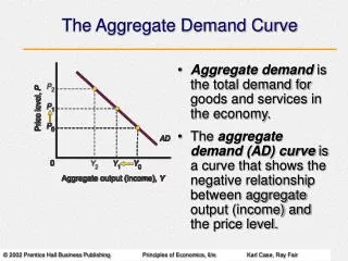
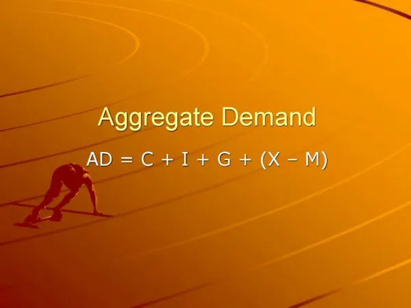
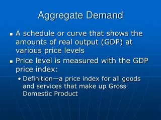
Aggregate Demand • Aggregate demand is the total demand in an economy for all the goods and services produced. • The aggregate demand schedule is a schedule relating the total demand in an economy for all the goods and services to the price level. • Aggregate demand with aggregate supply determines the price level.
Aggregate Demand Curve • The aggregate demand curve slopes down. • As the general price level rises, the amount of goods and services that are produced decreases. • How can we better understand this concept? • Economic theory.
Money Demand • Money yields a flow of exchange services that increase the convenience of buying and selling goods and services. • Marginal benefit of holding money is the usefulness of having ready cash. • Marginal cost of holding money is the opportunity cost associated with not buying goods and services.
Budget Constraint: Barter Economy • PYD = Pp + wLS • where • PYD = Demand for Commodities • Pp = Profit • wLS = Labor Income • In this economy, no money changes hands and no family uses money for trade, but money can be used as a unit of account.
Budget Constraint: Monetary Economy • MD + PYD = p + wLS + MS • where • MD = Money Held at the End of the Period • PYD = Demand for Commodities • p = Profit • wLS = Labor Income • MS = Money Supplyat the Beginning of the Period
Budget Constraint: Classical Model • MD + PYD = p + wLS + MS • MS acts like additional income that is available to buy commodities. • MD represents the money people do not spend during the period. It is the amount they set aside for future purchases. • The decision to hold money idle imposes an opportunity cost on people equal to the additional utility that could be gained by purchasing commodities.
Money Demand: Classical Model • Classical economists argued that the stock of money that the average household needs at any moment in time is directly proportional to the dollar value of its demand for commodities. • MD = k x PYD • where k is the factor of proportionality.
The Cambridge Equation • MD = kPYD is a demand for money theory known asthe Cambridge equation. • Money demand is some fraction (k) of total nominal output. • Money demand is determined only by income. • People hold this money in anticipation of the exchanges they will make in the near future. • They allocate the rest of their income to immediate consumption of goods and services.
Aggregate Demand: Classical Model • MD = kPYD • MD =MS • kPYD = MS Equilibrium Condition • Solve for P • MS /k = PYD Divide both sides by k • MS /kYD = P Divide both sides by YD
Aggregate Demand • P = MS/(kYD) • The equation shows how the price level is related to GDP, when money demand just equals money supply. • Note the inverse relationship between Y and P. • Along any single aggregate demand curve, money supply is constant. • Classical economists also assumed that k was a constant, determined by institutional factors.
The Quantity Theory of Money • The quantity theory relates the price level to the quantity of money circulating in an economy. • According to the Equation of Exchange, • MV = PY • Money supply times its velocity equals nominal GDP. • MD = MS • Money demand equals money supply at equilibrium. • MD = (1/V)PY = MD = kPY • Money demand is proportional to nominal GDP. • P = (MS1/k)/Y = MS/kYD • Aggregate demand curve at equilibrium.
Irving Fisher and Velocity • V = PT/MS • The velocity of circulation just equals the average value of transactions divided by the nominal money supply. • T = YD • V = PYD/MS • P = VMS/YD • Since V = 1/k, Fisher’s version of the relationship between the price level and GDP is identical to that of the Cambridge equation and the quantity theory.
Aggregate Demand Curve At every point on the AD curve, the demand for money just equals money supply. In addition, the nominal value of GDP (PxY) is constant. Classical economists also assumed that k was a constant. The aggregate demand curve slopes downward because as the price level falls people have more money on hand to buy goods and services. P P2 P1 AD 0 Y1 Y2 Y
Equilibrium AS P The equilibrium price level ensures that the amount of real output that individuals wish to purchase, given the quantity of money and the income velocity of money, is equal to the level of real output produced by firms. AD 0 Y
Shifting Aggregate Demand • Two factors shift aggregate demand • Changes in the money supply • Increases shift AD to the right. • Decreases shift AD to the left. • Changes in k • Decreases in k shift the AD to the right. • Increases in k shift the AD to the left.
Aggregate Demand P Shifts in aggregate demand are caused by changes in the money supply or changes in the velocity of money. An increase in money or a decrease in k shifts AD to the right. A decrease in money or an increase in k shifts AD to the left. AD3 AD2 AD1 0 Y
Aggregate Demand and Aggregate Supply: Math • Previous results: YS = LD – (½ )(LD)2Production function 1 – LD = (w/P) Labor demand LS = (w/P) Labor supply (w/P)E = ½ Equilibrium real wage LE = ½ Equilibrium labor YE = 3/8 Equilibrium output
Aggregate Demand and Aggregate Supply: Math • Let k = 2 and MS = 100. • P = MS/kYE • P = 100/2 x (3/8) = 133.33 • (w/P)E = ½ • wE = PE x ½ = 66.66
Implications of the Classical AD/AS Model • There are four implications that can be drawn from the long-run aggregate demand/aggregate supply model. • Full employment prevails: Recessions and booms must be temporary. • Changes in aggregate demand have no impact on output and employment. • Inflation is a monetary phenomenon. • Supply is the key to growth.
Full Employment Prevails • The classical model is characterized by the process of market clearing. • Surpluses and shortages are short run, transitory events that are corrected by price changes that re-equilibrate the relevant markets. • Recessions and booms are temporary and self-correcting.
Full Employment Prevails AS P If the price level is P3, excess supply of goods and services drives down prices until equilibrium is reached. If the price level is P1, excess demand for goods and services drives up prices until equilibrium is reached. P3 . P2 P1 AD Y 0 Y1 Y2 Y3
Changes in Aggregate Demand Have No Effect on Output or Employment • Shifts in aggregate demand change the price level, but cannot change the level of output. • An increase in aggregate demand causes the price level to rise. Prices rise until the original equilibrium level of Y is restored. • A decrease in aggregate demand causes the price level to fall. Prices fall until the original equilibrium level of Y is restored.
Aggregate Demand and Employment AS P An increase in aggregate demand causes the aggregate demand curve to shift to the right. At C, demand exceeds supply causing the price level to rise. P2 B A C P1 AD2 AD1 0 Y1 Y
Y=F(L) Y Y Y1 L Y 0 0 Y1 P w/P LS 1 W/P1 P2 2 3 W/P2 AD2 P1 AD1 LD 0 Y 0 L Y1 LS LD
Aggregate Demand • Increases in the aggregate demand curve cause prices to begin to rise. • As P rises, the real wage falls, encouraging firms to hire more workers. • But, the decrease in the real wage also causes workers to decrease labor supply. • The nominal wage, w, rises until labor demand just equals labor supply. • Output remains constant. In equilibrium, only the price level increases.
Policy Implication • Macroeconomic stabilization policies are powerless. • Government spending and/or taxing policies typically are designed to shift aggregate demand rather than aggregate supply and so are powerless to change economic conditions in the classical model. • Why?
Inflation is Caused by the Central Bank • Inflation is a sustained rise in the overall price level. • In the classical model, the price level rises when AD shifts to the right . • Given constant velocity, aggregate demand shifts only when the money supply changes. • Therefore, the central bank causes inflation with excessive monetary growth.
Money, Output, and Inflation AS P An increase in the money supply causes the aggregate demand curve to shift to the right. At C, demand exceeds supply causing the price level to rise. P2 B A C P1 AD2 AD1 0 Y1 Y
Y=F(L) Y Y Y1 L Y 0 0 Y1 P W LS 6 W/P1 3 P2 2 4 5 W/P2 AD2 P1 1 AD1 LD 0 0 L Y Y1 LD LS
Money and Inflation • Inflation is a monetary phenomenon. • Aggregate demand shifts to the right as the money supply rises. Prices begin to rise. • As P rises, the real wage falls, encouraging firms to hire more workers. • But, the decrease in the real wage causes workers to decrease labor supply. • The nominal wage, w, rises until labor demand just equals labor supply. • Output remains constant. In equilibrium, only the price level increases.
Inflation and the Quantity Theory • MSV = PYS • /\MS/MS + /\V/V = /\P/P + /\YS/YS • /\P/P = /\MS/MS – /\YS/YS • The rate of inflation equals the rate of money supply growth minus the rate of output growth.
Policy Implication • Money does not influence real events in the classical model. • A change in the money supply shifts aggregate demand. • This begins a process of market clearing that ultimately results in the restoration of equilibrium at the initial level of Y coupled with a new price level. • Money is a veil = Money neutrality
Supply is the Key to Growth • Aggregate supply increases for two reasons: • New technology increases the productivity of each worker. • A higher real wage increases the number of laborers in the labor supply.
Supply is the Key to Growth P AS1 AS2 Economic growth causes the aggregate supply curve to shift to the right. At every price level, more is produced. Note that, other things remaining the same, an increase in aggregate supply results in a decrease in the price level A P1 B P2 AD 0 Y Y1 Y2
Y Y Y2=F(L) Y2 2 Y1=F(L) 1 Y1 0 L Y 0 P w/P AS2 AS1 LS 2 w2/P1 1 w1/P1 AD LD1 LD2 0 Y 0 L1 L Y1 Y2
Productivity Increase • New technology, more capital and better trained workers increase productivity. • The production function shifts up. • The labor demand curve shifts to the right. • The increase in demand for labor increases the real wage, causing an increase in labor supply along the labor supply curve. • Aggregate supply increases. • At the price level, P1, more output is produced.
Y Y Y=F(L) Y2 Y1 L Y 0 0 Y1 P w/P LS1 LS2 1 w1/P1 2 w2/P1 AD LD L Y 0 0 Y1Y2 L1 L2
Increase in Labor Supply • A change in worker preferences with respect to labor supply and an increase in the number of workers available shift the labor supply curve. • If workers decide to work more or the labor force expands, the labor supply curve shifts to the right. • The increase in labor supply decreases the real wage, causing firms to move down along the labor demand curve and hire more workers. • Equilibrium employment and aggregate supply increase.
Policy Implication • Government policies designed to influence economic activity should be carefully examined for their impact on labor demand and labor supply. • Tax changes can either increase or decrease labor supply. • Tax changes can either increase or decrease business incentives to invest in new capital.
Y=F(L) Y Y Y1 L 0 0 Y L1 w/P P LS w/P LD 0 0 L L1 Y
Y=F(L) Y Y Y1 L Y 0 0 Y1 P w/P LS w/P1 P1 AD1 LD 0 L Y 0 L1 Y1