Download
1 / 54
540 likes | 714 Vues
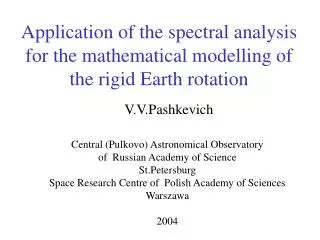
Construction of the Non-Rigid Earth Rotation Series. V.V. Pashkevich. Central (Pulkovo) Astronomical Observatory of the Russian Academy of Science St.Petersburg Space Research Centre of the Polish Academy of Sciences Warszawa 2007.

E N D
Construction of the Non-Rigid Earth Rotation Series V.V. Pashkevich Central (Pulkovo) Astronomical Observatory of the Russian Academy of Science St.Petersburg Space Research Centre of the Polish Academy of Sciences Warszawa 2007
The last years a lot of attempts to derive a high-precision theory of the non-rigid Earth rotation was carried out. For these purposes used the different transfer functions, which usually applied to the nutation in longitude and in obliquity of the rigid Earth rotation with respect to the ecliptic of date. Aim: Construction of a new high-precision non-rigid Earth rotationseries (SN9000), dynamically adequate to the DE404/LE404 ephemeris over 2000 years, which is expressed asa function of the three Euler angleswith respect to the fixed ecliptic plane and equinox J2000.0.
S T E P S: • The high-precisionnumerical solution of the rigid Earth rotation have been constructed (V.V.Pashkevich, G.I.Eroshkin and A.Brzezinski, 2004), (V.V.Pashkevich and G.I.Eroshkin, Proceedings of “Journees 2004”). The initial conditionshave been calculated from SMART97 (P.Bretagnon, G.Francou, P.Rocher, J.L.Simon,1998). The discrepancies between the numerical solution and the semi-analytical solution SMART97 were obtained in Euler angles over 2000 years with one-day spacing.
S T E P -1: Numerical integration of the differential equations Discrepancies: numerical solution minus SMART97 Initial conditions from SMART97
S T E P -1: Numerical integration of the differential equations Discrepancies: numerical solution minus SMART97 Initial conditions from SMART97 LAGRANGE DIFFERENTIAL EQUATIONS OF THE SECOND KIND: VECTOR OF THE GEODETIC ROTATION: Problem expressed by the Rodrigues – Hamilton parameters:
Fig.1 Numerical solution for Rigid Earth rotation minussolution SMART97 in the longitude of the ascending node of the Earth equator. Kinematical (relativistic) caseDynamical (Newtonian) case
Fig.2 Numerical solution for Rigid Earth rotation minussolution SMART97 in the angle of the proper rotation of the Earth. Kinematical (relativistic) caseDynamical (Newtonian) case
Fig.3 Numerical solution for Rigid Earth rotation minussolution SMART97 in the inclination angle. Kinematical (relativistic) caseDynamical (Newtonian) case
S T E P S: • The high-precisionnumerical solution of the rigid Earth rotation have been constructed (V.V.Pashkevich, G.I.Eroshkin and A.Brzezinski, 2004), (V.V.Pashkevich and G.I.Eroshkin, Proceedings of “Journees 2004”). The initial conditionshave been calculated from SMART97 (P.Bretagnon, G.Francou, P.Rocher, J.L.Simon,1998). The discrepancies between the numerical solution and the semi-analytical solution SMART97 were obtained in Euler angles over 2000 years with one-day spacing.
S T E P S: • The high-precisionnumerical solution of the rigid Earth rotation have been constructed (V.V.Pashkevich, G.I.Eroshkin and A.Brzezinski, 2004), (V.V.Pashkevich and G.I.Eroshkin, Proceedings of “Journees 2004”). The initial conditionshave been calculated from SMART97 (P.Bretagnon, G.Francou, P.Rocher, J.L.Simon,1998). The discrepancies between the numerical solution and the semi-analytical solution SMART97 were obtained in Euler angles over 2000 years with one-day spacing. • Investigation of the discrepancies is carried out by the least squares (LSQ) and by the spectral analysis (SA)algorithms (V.V.Pashkevich and G.I.Eroshkin, Proceedings of “Journees 2005”, 2005). The high-precision rigid Earth rotation series S9000is determined (V.V.Pashkevich and G.I.Eroshkin, 2005 ).
S T E P -1: Numerical integration of the differential equations Discrepancies: numerical solution minus SMART97 Initial conditions from SMART97 S T E P - 2
S T E P S-1 and 2: Numerical integration of the differential equations Discrepancies: numerical solution minus SMART97 Initial conditions from SMART97 Precession and GMSTtermsof SMART97 Calculation of the secularterms by the LSQ method Set of nutation terms of SMART97 Computationof the new precession and GMST parameters Removalof the secular trends from the discreapancies Calculation of the periodical terms by the SA method High-precision series S9000 Constructionof the newnutation series
Fig.4. The numerical solutionof the rigid Earth rotationminus S9000 after formal removal of the secular trends in the proper rotation angle. Kinematical caseDynamical case
Kinematical caseDynamical case Fig.5. Differences between S9000 andSMART97.
S T E P S: • The high-precisionnumerical solution of the rigid Earth rotation have been constructed (V.V.Pashkevich, G.I.Eroshkin and A.Brzezinski, 2004), (V.V.Pashkevich and G.I.Eroshkin, Proceedings of “Journees 2004”). The initial conditionshave been calculated from SMART97 (P.Bretagnon, G.Francou, P.Rocher, J.L.Simon,1998). The discrepancies between the numerical solution and the semi-analytical solution SMART97 were obtained in Euler angles over 2000 years with one-day spacing. • Investigation of the discrepancies is carried out by the least squares (LSQ) and by the spectral analysis (SA)algorithms (V.V.Pashkevich and G.I.Eroshkin, Proceedings of “Journees 2005”, 2005). The high-precision rigid Earth rotation series S9000is determined (V.V.Pashkevich and G.I.Eroshkin, 2005 ).
S T E P S: • The high-precisionnumerical solution of the rigid Earth rotation have been constructed (V.V.Pashkevich, G.I.Eroshkin and A.Brzezinski, 2004), (V.V.Pashkevich and G.I.Eroshkin, Proceedings of “Journees 2004”). The initial conditionshave been calculated from SMART97 (P.Bretagnon, G.Francou, P.Rocher, J.L.Simon,1998). The discrepancies between the numerical solution and the semi-analytical solution SMART97 were obtained in Euler angles over 2000 years with one-day spacing. • Investigation of the discrepancies is carried out by the least squares (LSQ) and by the spectral analysis (SA)algorithms (V.V.Pashkevich and G.I.Eroshkin, Proceedings of “Journees 2005”, 2005). The high-precision rigid Earth rotation series S9000is determined (V.V.Pashkevich and G.I.Eroshkin, 2005 ). • The new high-precision non-rigid Earth rotation series (SN9000),which expressed in the function of the three Euler angles, is constructed by using themethod (P.Bretagnon, P.M.Mathews, J.-L.Simon: 1999) and thetransfer function (Mathews, P. M., Herring, T. A., and Buffett B. A., 2002).
S T E P -3: Expressions for Euler angles:
Classical A l g o r i t h m Expressions for the non-rigid Earth nutations in longitude and obliquity:
TRANSFER FUNCTIONS J.M.Wahr ,1981; V. Dehant and P. Defraigne, 1997: T. Shirai and T. Fukushima, 2001:
TRANSFER FUNCTIONS P.Bretagnon, P.M. Mathews,J.-L. Simon,1999: P.M. Mathews, T.A. Herring, B.A. Buffett,2002:
TRANSFER FUNCTIONS P.M. Mathews, T.A. Herring, B.A. Buffett,2002: Geophisical model includes : The effects Electromagnetic coupling The Ocean effects Mantle inelasticity effects Atmospheric effects Change in the global Earth dynamical flattening and in the core flattening
Algorithm of Bretagnon et al. 1999 1.The rigid Earth angular velocity vector:
Expressions forthe Earth’s angular velocity vector: The coefficients of the developments of p, qin case of the rigid Earth:
The componentsofthe coefficients of the developments of p, q in case of the rigid Earth:
The amplitudes of the prograde and retrograde components: Complex transformation of the componets of the angular velocity vector:
Algorithm of Bretagnon et al. 1999 1.The rigid Earth angular velocity vector: 2.The non-rigid Earth angular velocity vector is obtained by:
The componentsofthe coefficients of the developments of p, q in case of the non-rigid Earth:
The progradeandretrograde components ofthe coefficients of the developments of pin case of the non-rigid Earth:
The progradeandretrograde components ofthe coefficients of the developments of qin case of the non-rigid Earth:
The sin coefficients ofthe developments for the non-rigid Earth angular velocity vector:
The cos coefficients ofthe developments for the non-rigid Earth angular velocity vector:
Algorithm of Bretagnon et al. 1999 1.The rigid Earth angular velocity vector: 2.The non-rigid Earth angular velocity vector is obtained by: 3.The derivatives of Euler angles for the non-rigid Earth rotation:
Common form of the periodic part of Euler angles: Cascade method:
Details: Iterative solution of the algorithm of Bretagnon et al. 1999 1 iteration
Details: Iterative solution of the algorithm of Bretagnon et al. 1999 n iteration Iterations are repeated until the absolute value of the difference between iterations K-1 and K exceedes some DEFINITE values
Results: Table 1. Comparison of different solutionsArgument (λ3 +D-F) with a 18.6 year period DD- Dehant and Defraigne, 1997; BMS- Bretagnonet al., 1999; SF-Shirai and Fukushima, 2001; MHB- Mathews et al.,2002.
Results: Table 1. Comparison of different solutionsArgument (λ3 +D-F) with a 18.6 year period DD- Dehant and Defraigne, 1997; BMS- Bretagnonet al., 1999; SF-Shirai and Fukushima, 2001; MHB- Mathews et al.,2002.
Table 2. Comparison of different solutionsFor some arguments SMN=SMART97+MHB; SN9000=S9000+MHB; MHB- Mathews et al.,2002.
Fig.6. The differences between SN9000 andSMN after removal of the secular terms. (non-rigid Earth rotation) Dynamical case μas Δφ Δθ Δψ YEARS
Fig.7. The differences between S9000 andSMART97 after removal of the secular terms. (rigid Earth rotation) Dynamical case μas Δφ Δθ Δψ YEARS
Fig.8. The differences between SN9000 andSMN after removal of the secular terms. (non-rigid Earth rotation) Kinematicalcase μas Δφ Δθ Δψ YEARS
Fig.9. The differences between S9000 andSMART97 after removal of the secular terms. (rigid Earth rotation) Kinematicalcase μas Δφ Δθ Δψ YEARS
Fig.10. The differences between S9000 andSN9000. Dynamical case μas Δφ Δθ Δψ YEARS
Fig.11. The differences between S9000 andSN9000. Kinematicalcase μas Δφ Δθ Δψ YEARS
Fig.12. The differences between SMART97 andSMN. Dynamical case μas Δφ Δθ Δψ YEARS
Fig.13. The differences between SMART97 andSMN. Kinematicalcase μas Δφ Δθ Δψ YEARS
Fig.14. The discrepancies between S9000 andSN9000minusdiscrepanciesbetween SMART97 andSMN. Dynamical case μas Δφ Δθ Δψ YEARS
Fig.15. The discrepancies between S9000 andSN9000minusdiscrepanciesbetween SMART97 andSMN. Kinematicalcase μas Δφ Δθ Δψ YEARS