Understanding the Consumption Function in Aggregate Demand Analysis
This presentation explores the consumption element of aggregate demand, focusing on the consumption function, which illustrates the relationship between income and consumer expenditure. According to Keynesian theory, household spending is linked to disposable income. Key concepts such as autonomous spending and the marginal propensity to consume (MPC) are discussed, alongside factors influencing shifts in the consumption function, including interest rates, household wealth, and consumer confidence. The presentation is accessible on the G13 Wiki for further learning.


Understanding the Consumption Function in Aggregate Demand Analysis
E N D
Presentation Transcript
Deconstructing Aggregate Demand This presentation will go through the Consumption element of Aggregate Demand. It will be made available on the G13 Wiki http://ib-econ-dubai-2011-12.wikispaces.com/
Consumption • The consumption functionThe consumption function is simply a theoretical relationship between income and consumer expenditure. The Keynesian theory describes a consumption function where household spending is directly linked to people’s disposable income. A simplified consumption function diagram is shown below
Diagram showing Consumption function Consumer Spending Consumption = Disposable Income C2 C1 C3 Change in Consumption Change in Income a 450 line Disposable Income $ Billion
Some Math! • The standard Keynesian consumption function is written as follows:C = a + c (Yd) – where • C is total consumer spending • a is autonomous spending • And c (Yd) is the propensity to spend out of disposable income • Autonomous spending (a) is consumption which does not depend on the level of income. For example people can fund some of their spending by using their savings or by borrowing money from banks and other lenders. A change in autonomous spending would in fact cause a shift in the consumption function leading to a change in consumer demand at all levels of income. • The key to understanding how a rise in disposable income affects household spending is to understand the concept of the marginal propensity to consume (mpc). The marginal propensity to consume is the change in consumer spending arising from a change in disposable income. If for example your disposable income rises by $5,000 and you choose to spend $3000 of this on extra goods and services, then the mpc is $3000/$50000 or 0.66. If you chose instead to spend only $2500 of the increase in income, then the mpc would be 0.5. • The gradient of the consumption function shown in the previous diagram is determined by the value for marginal propensity to consume. A change in the mpc (shown in the next diagram) would cause a pivotal change in the consumption function. For example, a decision to save less of any increase in income would lead to a rise in the mpc and a steeper consumption curve.
Shifts in the Consumption Function Consumer Spending Consumption = Disposable Income Consumption =a2 +c(Yd) Consumption =a +c(Yd) a2 a 450 line Disposable Income $ Billion
Shifts in the Consumption Function • A change in any factor affecting consumption other than a change in income is said to lead to a shift in the consumption function. These factors include the following: • A change in interest rates – for example a cut in interest rates will boost consumption at each level of income and cause an upward shift in the consumption function. Lower interest rates act to lower the cost of servicing the debt on a mortgage and thereby increase the effective disposable incomeof homeowners. In contrast a period of higher interest rates is designed to curb consumer spending. • A change in household wealth – for example a rise in house prices or in share prices encourages higher levels of borrowing and an upward movement in the consumption curve. • A change in consumer confidence – for example, expectations of rising unemployment and worsening expectations of changes in income might lead to a reduction in confidence and a fall in spending at each level of income. Conversely an improvement in consumer expectations about the health of the economy will increase confidence and planned spending. • Consumer spending in Britain had grown consistently strongly up to 2008, but the credit crunch, financial crises & restrictive fiscal policies has seen the first decrease in household disposable income since the 1970’s.
Disposable Income • In our example above, as disposable income rises in blocks of $10,000, so does total consumption. But the rate at which consumer spending is increasing is declining. The marginal propensity to consume is falling and this brings down the average propensity to consume.The Keynesian theory did actually argue that the marginal propensity to consume would fall as income increases, but the evidence for the UK over many years disputes this – perhaps people were spending more than their current disposable income? How is this possible?
The Savings Function We assume that any disposable income that is not spent is saved, so we can deduce from our numerical example above, that because the marginal propensity to consume is falling, then the marginal propensity to save must be rising as is the average propensity to save (otherwise known as the household savings ratio). This is shown in the savings function table which is drawn from the data on consumption and income used in the first table.
Alternative Theories of Consumption The life—cycle model The life-cycle model of consumption was developed by Franco Modigliani who argued that households form a view about their likely or expected income over a large slice of their life-cycle, and then base their spending decisions around this. This helps to explain why people in reasonably well paid jobs in their early twenties are prepared to borrow heavily to finance current consumption (a new car, furnishings for a property) because they expect to be able to repay loans as their disposable income increases. Similarly people reaching middle age frequently tend to become net savers because they are anticipating saving for their retirement. One of the results of the life-cycle model is that changes in the age structure of the population can have sizeable effects on total consumer spending in the economy.
Alternative Theories of Consumption The permanent income modelThis model of consumption is associated with the US economist Milton Friedman and it is, in many ways, a development of the life-cycle mode. Friedman believed that people base their spending decisions on expectations of permanent income. Permanent income might be described as the average income that people can earn over their lifetime. A distinction is made between transitory income (e.g. a windfall gain in income which has not been earned) and permanent income. Friedman believed that changes in transitory income would not fundamentally affect spending and saving decisions. But that shifts in permanent income would be important in shaping our spending levels. • For example, a rise in household wealth increases the ability of people to spend perhaps through borrowing secured on the value of a property. Lower interest rates tend to increase both share and house prices adding to household wealth. That said lower interest rates also cut the income flowing to people with net savings. • According to the permanent income model, only changes in permanent income have any long term effect on consumption. But transitory changes in spending power can lead to a more volatile pattern for the propensity to consume.
Homework • Blink & Dorton • Read pages 170-179 • On P179 answer student work point 14.6 • Answer all 3 questions on Germany • E-mail me or hand in on Sunday 9th P4. dlsocmbe@eischools.ae Thank you for following this presentation