XAFS: X-ray Absorption Fine-Structure

1. XAFS: X-ray Absorption Fine-Structure Matt Newville Consortium for Advanced Radiation Sources University of Chicago / Advanced Photon Source Overview of XAFS and XANES XAFS experiment design: transmission and fluorescence Fe foil, FeO, Fe2O3, Fe in cytochrome-c Data Analysis overview Today: Lecture (1 hour) XAFS measurements at 20-BM in groups of 5 (~1 hour/group). Data Analysis on example and measured data. Tomorrow: XAFS measurements (if needed) Data Analysis on example and measured data.

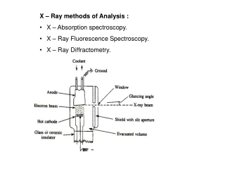
2. X-ray Absorption Spectroscopy: Measure energy-dependence of the x-ray absorption coefficient m [either log(I0 /I) or (If / I0 )] for an atomic core-level electron of a selected element. X-ray Absorption Spectroscopy Transmission Measurements: Measured x-ray beam intensities for I0 (left) and I (right)

3. X-ray Absorption Fine Structure (XAFS) We’re interested in the oscillations in m(E):

4. X-ray Absorption: Atomic View An atom absorbs and x-ray of energy E, destroying a core electron with energy E0 and creating a photo-electron with energy (E-E0). The core level is refilled and a fluorescence x-ray or an Auger electron is ejected from the atom. absorption requires an available electronic state for the photo-electron. No available state: No absorption by that core level For an isolated atom, m(E) is a smooth function of energy.

5. X-ray Absorption Fine-Structure Spectroscopy With another atom nearby, the photo-electron can scatter from the neighbor atom. The interference of the outgoing and scattered waves alters the photo-electron wave-function at the absorbing atom, modulating m(E). The absorption probability m(E) depends on the spatial overlap of the core-level and photo-electron wave-functions. The core-level is localized, so the overlap is determined by the photo-electron wave-function at the absorbing atom. The interference of outgoing and scattered photo-electron gives the oscillations in m(E)

6. X-ray Absorption Spectroscopy: Measure energy-dependence of the x-ray absorption coefficient m(E) [either log(I0 /I) or (If / I0 )] of a core-level of a selected element X-ray Absorption Spectroscopy: Why Bother? Element Specific: Elements with Z>20 can have EXAFS measured at the APS. Valence Probe: XANES gives chemical state and formal valence of selected element. Local Structure Probe: EXAFS gives atomic species, distance, and number of near-neighbor atoms around a selected element.. Low Concentration: concentrations down to 10 ppm for XANES, 100 ppm for EXAFS. Natural Samples: samples can be in solution, liquids, amorphous solids, soils, aggregrates, plant roots, surfaces, etc. Samples do not need to be crystalline. XANES = X-ray Absorption Near-Edge Spectroscopy EXAFS = Extended X-ray Absorption Fine-Structure

7. The EXAFS Equation EXAFS: the fine-structure oscillations in m(E) where k is the photo-electron wavenumber: The EXAFS results from an outgoing photo-electron scattering from a neighbor atom, and returning to the core atom to interfere with the core level: Outgoing photo-electron Scattering from neighbor atom (amplitude and phase depend on Z of neighbor atom) Returning photo-electron

8. The EXAFS Equation Photo-electron scattering The EXAFS Equation for 1 atomic site (no disorder) Averaging over all atoms in the sample, which has a distribution of distances (including structural and thermal disorder) the EXAFS Equation becomes: s2 = mean-square disorder in R This fairly simple equation allows us to model near-neighbor species - through f(k) and d(k) – and distance R, and coordination number N .

9. X-ray Absorption Measurements: Experimental Design Important points to consider for measuring XAFS are: Monochromatic x-rays:Need x-rays with a small energy spread or bandwidth. ~1eV at 10keV Linear Detectors:The XAFS c(k) is ~10-2 or smaller, so we need a lot of photons (ie, a synchrotron) and detectors that are very linear in x-ray intensity (ion chambers). Well aligned Beam:The x-ray beam hitting the detectors has to be the same hitting the sample. Homogeneous sample:No pinholes, and having a uniform and appropriate sample thickness (for transmission) of ~2 absorption lengths.

10. X-ray Absorption Measurements: The Experiment Energy Scanning:The beamline needs to deliver monochromatic x-rays that are tunable so that we can scan energy across the absorption edge. We’ll scan from ~200eV below to ~800eV above the Fe K-edge, like this: Pre-edge ( -200 to –20eV ): 5.0eV steps. Edge ( -20 to + 20eV ): 0.5eV steps EXAFS ( +20 to ~800eV): 0.05 A-1 (photo-electron wavenumber) Counting statistics for Good Data: The EXAFS is fairly small, so m(E) should have a noise level of about 10-3. That means we need to collect ~ 106 photons. Transmission mode: no problem ( ~108 photons/sec) Fluorescence mode: may be a concern.

11. X-ray Absorption Measurements: Transmission For a concentrated sample (ie, most absorption is from the element of interest), XAFS is best measured in transmission. We need to get enough transmission through the sample to get a decent signal in the ion chamber. With, We adjust the sample thickness x so that above the absorption edge. For Fe foil: But: the sample must be uniform, and free of pinholes. If a transmission experiment can be done, this is an easy measurement and gives very good data.

12. X-ray Absorption Measurements: Fluorescence For dilute atoms (say, in solution, or at low concentration) , the matrix may absorb most of the x-rays, and we don’t get much change in transmission for the element we care about. XAFS can also be measured by monitoring the characteristic fluorescence from the excited atom. The measurement is different, but we analyze the resulting m(E) in exactly way the same as for transmission. For Fe K-edge, we’ll measure the Ka fluorescence line at 6.40keV. But: There will also be elastic and inelastic scatter that we don’t want:

13. X-ray Fluorescence X-ray Absorption X-ray Fluorescence Incident x-ray is destroyed. Core-level electron destroyed. Photo-electron ejected from atom. Higher energy core electron fills empty electron level, and ejects an x-ray of fixed energy. Ka : L electron fills K hole Kb : M electron fills K hole

14. X-ray Absorption Measurements: Fluorescence To separate the Ka fluorescence line at 6.40keV from the elastic scatter at ~7.10keV, we’ll use a filter of Mn: with an absorption edge at 6.5keV, it will absorb the scatter much more than the Fe Ka line. To prevent too much Mn Ka from getting in the detector, we’ll use a set of slits. Another common approach is to use a detector with energy discrimination to select the fluorescence line of interest.

15. XAFS Analysis I: Data Reduction No matter how we measure m(E), we’ll want to reduce this data to c(k), where k is the photo-electron wave number (momentum): 1: convert measured intensities to m(E). 2: subtract a pre-edge background and scale m(E) to go from 0 to 1. 3: remove a post-edge smooth background function m0(E) to isolate the XAFS: 4: weight XAFS and Fourier transform from k to R space. 5: Model f(k) and d(k) and analyze c(k) to get distances R, and coordination number N .

16. XAFS Data Reduction 1: convert measured intensities to m(E). I0 I

17. XAFS Data Reduction 2: subtract a pre-edge background and scale m(E) to go from 0 to 1. Fit a line in the pre-edge region and Fit a polynomial in the post-edge, and determine the edge jump.

18. XAFS Data Reduction 3: remove a post-edge smooth background function m0(E) to isolate the XAFS: Fit a smooth polynomial spline to the XAFS to remove the slowly varying (low-frequency) components of m(E) Edge Step

19. XAFS Data Reduction 4: weight XAFS and Fourier transform from k to R space. The XAFS is multiplied by k2 and then multiplied by a smoothing window function to eliminate ripple from truncation of c(k). Because of the d(k) term, the peaks in |c(R)| are not at the interatomic distances, but are shifted down by ~0.5A or so.

20. XANES: oxidation state identification X-ray Absorption Near-Edge Spectroscopy (XANES) is one of the only techniques that gives a direct measurement of chemical state (valence state) of an element. In many chemical and environmentally relevant systems, the valence state is as important as the total concentration of an element. XANES Analysis is somewhat more qualitative than EXAFS Analysis. There is a shift of the absorption edge by ~3eV per formal oxidation state for Fe, and qualitative differences in line shape.

21. XAFS Analysis II: Modelling c(k) The XAFS for a coordination shell is modelled using Where and are the photo-electron scattering factors. These are non-trivial functions, and we’ve calculated them using an Ab initio program called FEFF. Once we have these, we can get and We’ll also adjust these parameters in the analysis: Mean-square disorder in R Amplitude reduction factor Energy origin to define where

22. XAFS Analysis II: Modelling c(k) Sum over Paths The XAFS for a coordination shell is modelled using And we now Sum over Scattering Paths to get the full XAFS, with Contributions from all neighboring atom types and distances: Now and are calculated for each scattering path or coordination shell. The Parameters N, R, s2 are now extended for each Path. We’ll use 2 to 4 paths for most of the analysis here.

23. XAFS Analysis With G.I.Feffit To Start the XAFS Analysis Program, click on the G.I.Feffit icon: The example data and analysis scripts are in C:\IFEFFIT\NXS\ G.I.Feffit will start in that directory, At the command line, type ‘cd Fe’ to move to the Fe subdirectory. From the menus, pick File->Read Command File and Choose Analyze.iff. Single Step through this script to see the steps involved in reducing raw data All the way to The command file Fit.iff will define the FEFF paths and fit the first shell of Fe metal.