Argo Delayed-Mode Process
Argo Delayed-Mode Process. Annie Wong University of Washington. Argo data quality control elements. Real-time (RT) data stream Function: Apply agreed RT QC tests to float data. Assign quality flags. Users: Operational centres, data assimilation, researchers needing timely data.

Argo Delayed-Mode Process
E N D
Presentation Transcript
Argo Delayed-Mode Process Annie Wong University of Washington
Argo data quality control elements Real-time (RT) data stream Function: Apply agreed RT QC tests to float data. Assign quality flags. Users: Operational centres, data assimilation, researchers needing timely data. Timeframe: 24-48 hrs after transmission. Who/Where: Perform by National Data Assembly Centres. Data from floats Delayed-mode (DM) data stream Function: Apply accepted DM procedures to float data. Provide statistically justified corrections using accepted methods. Provide feedback to RT system. Users: All needing adjusted data with error estimates. Timeframe: 6-12 months after transmission. Who/Where: Perform by PIs.
Introduction •Argo delayed-mode procedures are applied to 3 measurement parameters: PRES, TEMP, PSAL. •There is currently no recommended qc method for other auxiliary parameters, such as DOXY, that are reported in the Argo netCDF files.
Delayed-mode procedure for PRES 1).Check PRES by visual assessment of ensemble vertical profile plots of TEMP vs PRES and PSAL vs PRES. Assessment aims to identify anomalies that cannot be detected by the real-time qc tests on single profiles.
Example 1. Bad pressure sensor calibration coefficient. This will show up as anomalous T-S curve at depth when compared with nearby data.
Example 2. Druck pressure sensor problem, which can be identified when profiles become more and more shallow. Pressure measurements are erratic and suspect.
2). Adjust PRES using “SURFACE PRESSURE” if there is evidence that the values reported in “SURFACE PRESSURE” represent pressure sensor drift. Examine time series. Use next cycle “SURFACE PRESSURE” to adjust pressure. Then re-calculate salinity.
Delayed-mode procedure for TEMP Check TEMP by visual assessment of ensemble vertical profile plots of TEMP vs PSAL and TEMP vs PRES. Assessment aims to identify anomalies that cannot be detected by the real-time qc tests on single profiles.
Delayed-mode procedure for PSAL 1).Identify anomalies that cannot be detected by the real-time qc tests on single profiles. Example. Salinity “hooks” at base of profiles in some Apex floats (e.g. 590030), which often occur when two measurements are reported at nearly identical pressures.
2).Apply conductivity cell thermal mass correction. See Johnson, Toole, Larson (paper accepted in JAOT) Correction reduces spikes at base of mixed layers and shifts salinity towards saltier values in strong temperature gradients.
3).Check for sensor drift and calibration offset in salinity data. Apply statistical adjustments. Conductivity cells sometimes get contaminated, or experience electrical problems, that give measurements with artificial trends. OFFSET DRIFT θ θ S S
How to calibrate salinity data in the absence of an absolute reference? ► Use reference data to estimate salinity at float locations. ► Compare float salinity time series with reference time series. ► Evaluate. ► Apply statistical adjustment if needed.
Both schemes use the objective mapping method and its formal error estimates described by Bretherton et al (1976), in a two-step manner based on Roemmich (1983). Both schemes weight their salinity mapping by using a set of spatial decorrelation scales and a set of temporal decorrelation scales. Both schemes uses weighted least squares fit in potential conductivity space. • Wong, Johnson, Owens (2003) • anisotropic spatial decorrelation scales • CFC apparent ages • rotation of axes of the x-y coordinates to parallel the continental slope • pre-fixed standard θ levels • correction for each profile is obtained by weighted least squares fit in a “running window”. • error estimates take into account lateral and vertical data dependency. • Boehme, Send (2005) • uniform sptial decorrelation scales • moorings data • potential vorticity as a weighting factor • 10 “best” float observed levels • correction for each profile is obtained by fitting a line through a series of one-to-one fits over the lifetime of the float. • error estimates assume data are independent in the lateral and vertical.
An integrated scheme by Owens and Wong • Builds on WJO and the Böhme & Send formulations. • Assumes that the drift is piece-wise linear. Continuity is enforced unless the user splits the float series. • Chooses the statistically simplest model that fits the observed drift. • Uses horizontal and vertical correlations to estimate the effective number of degrees of freedom and a Monte Carlo simulations to estimate uncertainties.
Comparison example 1. This is a Scripps float from the Pacific. WJO (top panel) shows sensor drift, but the trend is not obvious until about cycle 60. Debate whether to split the series at cycle 60. OW (bottom panel) optimal fit suggests that the drift trend is continuous from the beginning of float life, therefore no split series is needed.
Comparison example 2. This is a UW float from the Pacific. WJO (top panel) shows sensor drift starting early on in float life. Visual inspection suggests sensor drift starts around cycle 15. OW (bottom panel) optimal fit confirms that sensor drift starts at cycle 15 by assigning a break point there. The remaining piecewise linear fit is similar to the WJO running window fit.
How to distinguish sensor drift from ocean variability? Examine salinity time series on multiple isotherms. Examine salinity anomaly time series over the full sampling depth. Salinity on isotherms will vary either (a) because of genuine changes of water mass properties observed as float migrates or as the ocean changes with time, or (b) because of sensor drift.
Genuine changes in water mass properties will be seen as a shift in salinity anomaly at some levels only. Sensor drift will be seen as a change in salinity anomaly at all levels.
How to minimize ocean variability in the statistical adjustment? Select 10 “best” surfaces to obtain differences between float measurements and reference data:- • Minimum S variance of (nearly constant) θ surfaces • Minimum P variance of (nearly constant) θ surfaces • Minimum S variance on P levels (4 levels) • Minimum θ variance on P levels (4 levels) Weighted least squares fit = inverse of mapping variance
Scientific decision:- Restricted the calibration range to 9°C < θ < 12°C.
What are the reference datasets? All post-1985 CTD data from WOD 2001 World Ocean Database + Additional recent CTD data Need datasets with:- • good quality data; • good spatial coverage; • recent in time.
Where to find Argo delayed-mode data? Real-time data Adjusted data PARAM_ADJUSTED PARAM_ADJUSTED_QC PARAM_ADJUSTED_ERROR PARAM PARAM_QC