Download
1 / 20
200 likes | 312 Vues
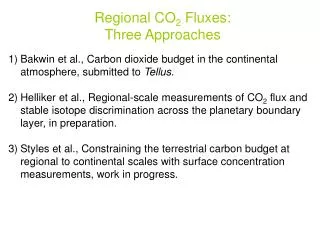
Regional CO 2 Fluxes: Three Approaches. Bakwin et al., Carbon dioxide budget in the continental atmosphere, submitted to Tellus . Helliker et al., Regional-scale measurements of CO 2 flux and stable isotope discrimination across the planetary boundary layer, in preparation.

E N D
Regional CO2 Fluxes:Three Approaches • Bakwin et al., Carbon dioxide budget in the continental atmosphere, submitted to Tellus. • Helliker et al., Regional-scale measurements of CO2 flux and stable isotope discrimination across the planetary boundary layer, in preparation. • Styles et al., Constraining the terrestrial carbon budget at regional to continental scales with surface concentration measurements, work in progress.
Gloor, M., et al., What is the concentration footprint of a tall tower? J. Geophys. Res., 106, 17831-17840, 2000.
Approach #1: Bakwin et al. Atmospheric budget on a monthly time scale. ∂CO2/∂t = Fc/Zmix – Ui (∂CO2/∂Xi)
Approach #2: Helliker et al.Boundary layer cuvette Where does this come from? The Lagrangian budget equation is: but … this is a Lagrangian equation advection has been ignored!
Approach #3: Styles et al.Uncalibrated flux sites • T is a period of time which starts in the morning before CBL growth begins, and ends in the afternoon when the CBL is fully developed • cB is CO2 within the CBL • c+ is CO2 above the CBL • h = zi (CBL height)
Approach #3: Styles et al.Uncalibrated flux sites • Wait a minute, is this right??? • What about the initial state of the CBL? (h ≠ 0 at t = 0 !) • This assumes that CO2 above the CBL in the a.m. = c+ • Nevertheless, we forge ahead …
You could get (cB – c+) from accurate measurements at a tower (cB) and take c+ as equal to the MBL value. BUT, flux tower CO2 mixing ratios are usually not well calibrated! Hence, Styles et al. substitute: (cmin – cavg) for (cB – c+) where cmin and cavg are daily minimum and daily average CO2 measured at the flux tower. Whaaat??? That can’t work!
cmin – cavg = 0.915 (cB – c+) – 5.80, r2 = 0.89 cB – c+ cmin –cavg
cmin and cavg from 30 m tower data cB from 396 m tower data (daily min) c+ from MBL data
Conclusions • Three very different approaches, each with very dubious simplifying assumptions, all give some reasonable-looking results. • Are we just lucky? Stupid? Both?