Download
1 / 1
10 likes | 142 Vues
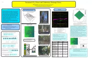
Fig. 4 : The main tower at the Harvard Forest. Fig. 1 : The topography at Harvard Forest. Note the exaggerated vertical scale. - determine whether measurable drainage flows exist. - evaluate whether these are connected to missed CO 2 fluxes.

E N D
Fig. 4: The main tower at the Harvard Forest Fig. 1: The topography at Harvard Forest. Note the exaggerated vertical scale. - determine whether measurable drainage flows exist - evaluate whether these are connected to missed CO2 fluxes - estimate magnitude of advective terms relative to eddy flux and storage Fig. 5: Inter-calibration of the anemometer array Fig. 2: The layout of the latest Draino Study. 2D: 2-dimensional sonic anemometer C#: inlet for horizontal CO2 gradient system Data Acquisition Hardware Links Fig. 6: One of the "satellite stations" consisting of 2-D sonic anemometer and CO2 inlet 3D Sonic Network Link to Albany Licor #1 Licor #2 23X PC, Linux Cyclades Operating Multi-Serial Port System 2D #1 2D #2 Dat Tape Zip Drive 2D #3 etc. Fig. 7: The "horizontal CO2 sampling system", based on a Licor7000 and a Valco rotary valve Fig. 3: Arbitrarily expandable serial data stream acquisition system Nocturnal CO2 Fluxes and Understory Drainage Flows Ralf M. Staebler*, David Fitzjarrald, Matt Czikowsky, Ricardo Sakai Atmospheric Sciences Research Center, SUNY Albany, NY *Corresponding Author: staebler@asrc.cestm.albany.edu AGU, December 2001 B51A-0176 Results Site and Measurements Objectives of this Research: The rate of change of a scalar c with source s is given by (1) After Reynolds’ decomposition and averaging, this can be expressed, simplified to 2 dimensions, as (2) advective terms flux divergence sources & sinks Assuming horizontal homogeneity, we can integrate vertically to z=h to obtain the eddy covariance flux equation most commonly used: (3) sources & sinks eddy flux at z=h storage term One objective is to look at some terms that are usually assumed to be zero: We can define horizontal advection (going back to 3D) as (4) (Vertical advection can be defined accordingly.) The continuity equation can be used to test the integrity of the data regarding mass flow: (5)