The climate model – ocean component
The climate model – ocean component. The Modular Ocean Model is designed primarily as a tool for studying the ocean climate system . But MOM has been used in regional and coastal applications , with many new features in mom4p1 aimed at supporting this work. Various options available

The climate model – ocean component
E N D
Presentation Transcript
The climate model – ocean component The Modular Ocean Model is designed primarily as a tool for studying the ocean climate system. But MOM has been used in regional and coastal applications, with many new features in mom4p1 aimed at supporting this work. Various options available -> flexibility, range of applications. (ie: Boussinesq approximation or Not) -> choice among various formulations: diffusion, vertical coordinate, equation of state, tracer packages ==> use of tables and namelists to turn on and off certain options/modules/parameterizations. Diagnostics/Tracer packages: Precipitation, steric sea level (changes in density) Temperature, FW, Ideal age tracer (time spent away from surface) CO2 Nutrients, chlorophyll, oxygen, helium, iron
Our MOM - Hydrostatic pressure - Non Boussinesq, changes in density - Finite Volumes method implemented on a b grid. conserves mass on each parcel, box sizes adjusted - Partial bottom cells, pressure coordinate - Fully non linear equation of state Jackett McDougall 2006 - Closed boundary conditions - 2 time steps- internal and external waves solved separately
Running the model Migrated to new cluster on campus. We have access to 10% of the resource (200cpu). HHPC V2 seems to be more reliable than previous version. Requires less babysitting! 1 run<=> requires 45cpu/200cpu available 1 year <=> 1h. How long can we afford to run sensitivity studies for? 1 year <=> 3Gb of storage. For long simulations, this might become an issue.
Initial and boundary conditions Model is initialized from previous run output. “Model data” or “Real data” SST and SSS from climatology or from atmospheric model FW flux (adds mass), River flow (estimated drainage from global river networks), runoff from land routed to an ocean discharge point, water injected into ocean over the top 40m. Ocean can be forced by atmospheric model outputs. Air-sea boundary forced by fluxes. For instance q=Precip-Evap+River+Ice Short wave radiation constant or varying seasonally. Chlorophyll or model-produced after SeaWIFS Coupled model provides heat flux, evaporation Models run for years, data averaged, extracted and passed as BC Lateral boundaries are closed unlike regional models. Basins have land boundaries on all lateral edges. Bottom kinematic boundary condition: no flow Surface : rigid lid: particle at the surface stays at the surface. Tidal forcing: 8 tidal constituents
What are we solving? T, S, SSH Density using the equation of state Pressure (hydrostatic—> comes after rho) Solve the momentum equation U, V Move water masses, update fields T, S, SSH Running the fully coupled model: atmosphere, ocean, ice, land Solves the equation of conservation of mass, momentum and tracers.
Finite Volume vs Finite difference Finite Volume vs Finite difference Finite Volume vs Finite difference Horizontal discretization: Differential or Integral equations of fluid motion solved usinge Finite Difference, Finite Element or Finite Volume methods. Finite element method: complex geometry, unstructured grids Finite volume method: is strictly conservative. Calculates fluxes. The budget for tracer mass per horizontal area is time stepped, not concentration. Finite difference method: does not strictly conserve mass. Truncation errors can be reduced by using higher order numerics. In practice, models can use FD for some eqn and FV for other. Equation of conservation of mass can be discretized with FV method even in a FD model while conservation of momentum will be discretized with FD method.
Fully non linear equation of state Fully non linear equation of state Fully non linear equation of state Fully non linear equation of state The equation of state in mom4p1 follows the formulation of Jackett et al. (2006) where the coefficients from McDougall et al.(2003b) are updated to new empirical data. density_insitu=f(Temperature,Salinity,pressure) Range: 0psu <= salinity <= 40 psu -3C <= theta <= 40C "theta" = either conservative or potential temperature 0dbar <= pressure <= 8000dbar
Bottom topography Generated from interpolation of satellite bathymetry, and heavily smoothed. User can open/close some boxes to better represent some features Tools exist to edit the bathymetry file. Drying or wetting boxes, moving straights around... How sensitive is the model to changes in bathymetry and coastaline? Data for validation? “ The topography used in OM3 was initially derived from a dataset assembled at the Southampton Oceanography Cen- tre for use in their global eddying simulations (A. Cow- ard, personal communication). This dataset is a blend of several products. Between 72◦ S and 72◦ N, version 6.2 of the satellite-derived product of Smith and Sandwell (1997) was mapped from the original Mercator projection onto a latitude-longitude grid at a resolution of 2 minutes. North of 72◦ N, a version of the International Bathymetric Chart of the Oceans (Jakobssen et al., 2000) was used, while south of 72◦ S the ETOPO5 product was used (NOAA, 1988).”
Tripolar grid Tripolar grid (Murray, 1996) to avoid the singularity at the north pole (coordinate transformation to a non spherical set of coordinates). Cross polar flows --> Paleoclimate: 1 ocean basin, interpolate bathymetry, what to do about thepolar singularity? Grid
Grid resolution Horizontal dimensions of the ocean grid vary according to latitude Higher resolution at the equator and mid latitudes Minimum latitudinal resolution at the equator is 0.6 degrees 28 vertical levels (aim is to represent equatorial thermocline and Subtropical planetary boundary layer) the uppermost eight of which are each 10 m thick layers gradually increase in thickness to a maximum of 506 m
Vertical coordinate The model employs partial bottom cells (Adcroft et al., 1997; Pacanowski and Gnanadesikan, 1998) to allow a more realistic representation of the bathymetry, with a maximum depth of 5500 m. Types of vertical coordinate in ocean model: Z-levels (Bryan). All grid points withing a given level are at the same depth - advantage: accurate pressure gradients are easy to calculate. - disadvantage: topo gradients are not well resolved at low resolution Isopycnal levels (Hallberg, Bleck, Smith). Lines of iso-density - advantage: approximate topo well - disadvantage: linear equation of state Sigma levels (Blumberg, Mellor, Haidvogel) - advantage: approximate topo well, coastal models - disadvante: pressure gradient errors, need corrections Partial bottom steps in MOM “piecewise-sigma” coordinate, p*=p_0b*(p-p_a)/(p_b-p_a) The model employs partial bottom cells (Adcroft et al., 1997; Pacanowski and Gnanadesikan, 1998) to allow a more realistic representation of the bathymetry, with a maximum depth of 5500 m. Types of vertical coordinate in ocean model: Z-levels (Bryan). All grid points withing a given level are at the same depth - advantage: accurate pressure gradients are easy to calculate. - disadvantage: topo gradients are not well resolved at low resolution Isopycnal levels (Hallberg, Bleck, Smith). Lines of iso density - advantage: approximate topo well - disadvantage: linear equation of state Sigma levels (Blumberg, Mellor, Haidvogel) - advantage: approximate topo well, coastal models - disadvante: pressure gradient errors, need corrections Partial bottom steps
Diffusion Vertical tracer diffusion Major role in determining the overall structure of the ocean circulation and its impact on climate. Changes in vertical diffusion can alter heat transport. Measurements estimate diffusivity K_v to be on the order of 0.1 to 0.15*e-4 m2/s in extra-tropical pycnocline (Ledwell et al 1993) Smaller values near the equator (Gregg et al 2003) Deep ocean: 1 to 2*e-4m2/s (Whitehead and Worthington 1982, Toole et al 1994, 1997) Difficulty to represent correctly the diapycnal diffusion
Diffusion There are 2 parts to the parameterization of lateral diffusion: - 1/ is to mix tracer properties along neutral surfaces by means of a diffusion operator oriented along the local isentropic surface (Redi 1982). The slope of the neutral direction relative to the surface of constant vertical coordinate is required to construct the neutral diffusion flux - 2/ is to adiabatically re-arrange tracers through an advective flux where the advecting flow is a function of slope of the neutral surfaces (Gent and McWilliams 1990). The advective flow is a function of the slope of neutral surfaces. Represents the transport effect of geostrophic eddies. Aredi 1000m2/s (much bigger than vertical diffusion coefficient) Agm