Partial Differential Equations: Classification, Examples, and Solutions
680 likes | 954 Vues
Learn about Partial Differential Equations (PDEs), their classification, important examples like the Laplace, Heat, and Wave Equations, and methods to solve them using Finite Difference Techniques. Dive into Parabolic Equations, Heat Conduction, Explicit and Implicit Methods, and the Stability of solutions. Enhance your knowledge in numerical methods for PDEs.

Partial Differential Equations: Classification, Examples, and Solutions
E N D
Presentation Transcript
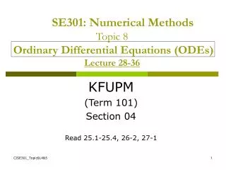
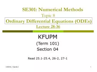
CISE301: Numerical MethodsTopic 9Partial Differential Equations (PDEs)Lectures 37-39 KFUPM (Term 101) Section 04 Read 29.1-29.2 & 30.1-30.4
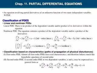
Lecture 37Partial Differential Equations Partial Differential Equations (PDEs). What is a PDE? Examples of Important PDEs. Classification of PDEs.
Partial Differential Equations A partial differential equation (PDE) is an equation that involves an unknown function and its partial derivatives.
Representing the Solution of a PDE(Two Independent Variables) • Three main ways to represent the solution T=5.2 t1 T=3.5 x1 Different curves are used for different values of one of the independent variable Three dimensional plot of the function T(x,t) The axis represent the independent variables. The value of the function is displayed at grid points
Heat Equation Different curve is used for each value of t ice ice Temperature Temperature at different x at t=0 x Thin metal rod insulated everywhere except at the edges. At t =0 the rod is placed in ice Position x Temperature at different x at t=h
Examples of PDEs PDEs are used to model many systems in many different fields of science and engineering. Important Examples: • Laplace Equation • Heat Equation • Wave Equation
Laplace Equation Used to describe the steady state distribution of heat in a body. Also used to describe the steady state distribution of electrical charge in a body.
Heat Equation The function u(x,y,z,t)is used to represent the temperature at time t in a physical body at a point with coordinates (x,y,z) is the thermal diffusivity. It is sufficient to consider the case = 1.
Simpler Heat Equation x T(x,t)is used to represent the temperature at time t at the point x of the thin rod.
Wave Equation The function u(x,y,z,t) is used to represent the displacement at time t of a particle whose position at rest is (x,y,z) . The constant c represents the propagation speed of the wave.
Classification of PDEs Linear Second order PDEs are important sets of equations that are used to model many systems in many different fields of science and engineering. Classification is important because: • Each category relates to specific engineering problems. • Different approaches are used to solve these categories.
Boundary Conditions for PDEs • To uniquely specify a solution to the PDE, a set of boundary conditions are needed. • Both regular and irregular boundaries are possible. t region of interest x 1
The Solution Methods for PDEs • Analytic solutions are possible for simple and special (idealized) cases only. • To make use of the nature of the equations, different methods are used to solve different classes of PDEs. • The methods discussed here are based on the finite difference technique.
Lecture 38Parabolic Equations Parabolic Equations Heat Conduction Equation Explicit Method Implicit Method Cranks Nicolson Method
Parabolic Problems ice ice x
Finite Difference Methods • Divide the interval x into sub-intervals, each of width h • Divide the interval t into sub-intervals, each of width k • A grid of points is used for the finite difference solution • Ti,j represents T(xi, tj) • Replace the derivates by finite-difference formulas t x
Solution of the Heat Equation • Two solutions to the Parabolic Equation (Heat Equation) will be presented: • 1. Explicit Method: • Simple, Stability Problems. • 2. Crank-Nicolson Method: • Involves the solution of a Tridiagonal system of equations, Stable.
Explicit MethodHow Do We Compute? T(x,t+k) T(x-h,t) T(x,t) T(x+h,t)
Convergence and Stability of the Solution • Convergence The solutions converge means that the solution obtained using the finite difference method approaches the true solution as the steps approach zero. • Stability: An algorithm is stable if the errors at each stage of the computation are not magnified as the computation progresses.
Example 1: Heat Equation ice ice x
Example 1 0 0 t=1.0 0 0 t=0.75 t=0.5 0 0 t=0.25 0 0 0 0 t=0 Sin(0.25π) Sin(0. 5π) Sin(0.75π) x=0.0 x=1.0 x=0.25 x=0.5 x=0.75
Example 1 0 0 t=1.0 0 0 t=0.75 t=0.5 0 0 t=0.25 0 0 0 0 t=0 Sin(0.25π) Sin(0. 5π) Sin(0.75π) x=0.0 x=1.0 x=0.25 x=0.5 x=0.75
Example 1 0 0 t=1.0 0 0 t=0.75 t=0.5 0 0 t=0.25 0 0 0 0 t=0 Sin(0.25π) Sin(0. 5π) Sin(0.75π) x=0.0 x=1.0 x=0.25 x=0.5 x=0.75
Example 1 – cont’d 0 0 t=0.10 0 0 t=0.075 t=0.05 0 0 t=0.025 0 0 0 0 t=0 Sin(0.25π) Sin(0. 5π) Sin(0.75π) x=0.0 x=1.0 x=0.25 x=0.5 x=0.75
Example 1 – cont’d 0 0 t=0.10 0 0 t=0.075 t=0.05 0 0 t=0.025 0 0 0 0 t=0 Sin(0.25π) Sin(0. 5π) Sin(0.75π) x=0.0 x=1.0 x=0.25 x=0.5 x=0.75
Example 1 – cont’d 0 0 t=0.10 0 0 t=0.075 t=0.05 0 0 t=0.025 0 0 0 0 t=0 Sin(0.25π) Sin(0. 5π) Sin(0.75π) x=0.0 x=1.0 x=0.25 x=0.5 x=0.75
Crank-Nicolson Method u(x-h,t) u(x,t) u(x+h,t) u(x,t - k)
Example 2 u1,4 u2,4 u3,4 0 0 t4=1.0 u1,3 u2,3 u3,3 0 0 t3=0.75 u1,2 u2,2 u3,2 t2=0.5 0 0 u1,1 u2,1 u3,1 t1=0.25 0 0 0 0 t0=0 Sin(0.25π) Sin(0. 5π) Sin(0.75π) x1=0.25 x3=0.75 x0=0.0 x2=0.5 x4=1.0
Example 2: Second Row at t2=0.5 sec u1,4 u2,4 u3,4 0 0 t4=1.0 u1,3 u2,3 u3,3 0 0 t3=0.75 u1,2 u2,2 u3,2 t2=0.5 0 0 u1,1 u2,1 u3,1 t1=0.25 0 0 0 0 t0=0 Sin(0.25π) Sin(0. 5π) Sin(0.75π) x1=0.25 x3=0.75 x0=0.0 x2=0.5 x4=1.0