Overview of EULAG: A Computational Model for Multi-Scale Fluid Dynamics
410 likes | 536 Vues
This document provides an overview of EULAG, the EUlerian/semi-LAGrangian numerical model designed for simulating fluid flows. Developed by Piotr K. Smolarkiewicz at the National Center for Atmospheric Research, EULAG integrates both Eulerian and Lagrangian approaches to fluid PDEs, employing advanced numerical algorithms such as Nonoscillatory Forward-in-Time (NFT) and preconditioned non-symmetric Krylov-subspace solvers. The model accommodates various fluid dynamics scenarios, from nonhydrostatic and compressible flows to turbulent dynamics, making it applicable in interdisciplinary settings.

Overview of EULAG: A Computational Model for Multi-Scale Fluid Dynamics
E N D
Presentation Transcript
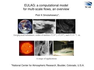
EULAG: a computational model for multi-scale flows, an overview Piotr K Smolarkiewicz*, *National Center for Atmospheric Research, Boulder, Colorado, U.S.A.
EULAG EUlerian/semi-LAGrangian numerical model for fluids Theoretical Features Two optional modes for integrating fluidPDEs: • Eulerian --- control-volume wise integral • Lagrangian --- trajectory wise integral Numerical algorithms: • Nonoscillatory Forward-in-Time (NFT) for the governing PDEs • Preconditioned non-symmetric Krylov-subspace elliptic solverGCR(k) • Generalized time-dependent curvilinear coordinates for grid adaptivity Optional fluid equations (nonhydrostatic): • Anelastic (Ogura-Phillips, Lipps-Hemler, Bacmeister-Schoeberl, Durran) • Compressible/incompressibleBoussinesq, • Incompressible Euler/Navier-Stokes’ • Fully compressible Euler equations for high-speed flows Note: not all options are user friendly ! Available strategies for simulating turbulent dynamics: • Direct numerical simulation (DNS) • Large-eddy simulation, explicit and implicit (LES, ILES)
Multi-time scale evolution of a meso-scale orographic flow(Smolarkiewicz & Szmelter, 2008, JCP, in press)
A Brief History • Early 1980’s (plus), development of MPDATA • Late 1980’s/early 1990’s, semi-Lagrangian advection and its extension on fluid systems • Early 1990’s, congruence of SL and EU and formulating GCR(k) pressure solver • Mid 1990’s, time-dependent lower boundary, extension to spheres (EulaS), parallelization • Late 1990’s/early 2000’s, unification of EULAG and EULAS • 2000’s , generalized coordinates and applications, unstructured meshes
Tenets of EULAG: Simplicity: a compact mathematical/numerical formulation Generality: interdisciplinary multi-physics applications Reliability: consistent stability and accuracy across a range of Froude, Mach, Reynolds, Peclet (etc.) numbers
Mathematical Formulation Multidimensional positive definite advection transport algorithm (MPDATA):
Abstract archetype equation for fluids, e.g., Eulerian conservation law Lagrangian evolution equation Kinematic or thermodynamic variables, R the associated rhs
Numerical design Either form (Eulerian/semi-Lagrangian) is approximated to second-order using a template algorithm: where is the solution sought at the grid point a two-time-level either advective semi-Lagrangian or flux-form Eulerian NFT transport operator (Sm. & Pudykiewicz, JAS,1992; Sm. & Margolin, MWR 1993).
Numerical design Motivation for Lagrangian integrals
Numerical design Motivation for Eulerian integrals Forward in time temporal discretization Second order Taylor sum expansion about t=nΔt Compensating first error term on the rhs is a responsibility of an FT advection scheme (e.g. MPDATA). The second error term depends on the implementation of an FT scheme
On grids co-locatedwith respect to all prognostic variables, it can be inverted algebraically toproduce an elliptic equation for pressure solenoidal velocity contravariant velocity Imposedon subject to the integrability condition Boundary conditions on Boundary value problemis solved using nonsymmetric Krylov subspace solver - a preconditioned generalized conjugate residual GCR(k) algorithm(Smolarkiewicz and Margolin, 1994; Smolarkiewicz et al., 2004) Numerical design All principal forcings are assumed to beunknown at n+1 system implicit with respect to all dependent variables.
Dynamic grid adaptivity Prusa & Sm., JCP 2003; Wedi & Sm., JCP 2004, Sm. & Prusa, IJNMF 2005 • A generalized mathematical framework for the implementation of deformable coordinates in a generic Eulerian/semi-Lagrangian format of nonoscillatory-forward-in-time (NFT) schemes • Technical apparatus of the Riemannian Geometry must be applied judiciously, in order to arrive at an effective numerical model. Diffeomorphic mapping (t,x,y,z) does not have to be Cartesian! Example: Continuous global mesh transformation
Boundary-fitted mappings; e.g., LES of a moist mesoscale valley flow (Sm. & Prusa, IJNMF 2005) Vertical velocity (left panel) and cloud water mixing ratio (right panel) in the yz cross section at x=120 km Cloud-water mixing ratio at bottom surface of the model
Boundary-adaptive mappings (Wedi & Sm., JCP, 2004) 3D potential flow past undulating boundaries Sem-Lagrangian option; Courant number ~5. Vorticity errors in potential-flow simulation
Boundary fitting mappings (Wedi & Sm., JCP, 2004) 3D potential flow past undulating boundaries Sem-Lagrangian option; Courant number ~5. mappings Vorticity errors in potential-flow simulation
Example: free-surface “real” water flow (Wedi & Sm., JCP,2004)
Urban PBL (Smolarkiewicz et al. 2007, JCP) tests robustness of the continuous mapping approach contours in cross section at z=10 m normalized profiles at a location in the wake
Model equations (intellectual kernel) Anelastic system of Lipps & Hemler (JAS, 1982)
Strategies for simulating turbulent flows • Direct numerical simulation (DNS), with all relevant scales of motion resolved, thus admitting variety of numerical methods; • Large-eddy simulation (LES), with all relevant sub-grid scales parameterized, thus preferring higher-order methods; • Implicit large-eddy simulation (ILES) — alias monotonically integrated large-eddy-simulation (MILES), or implicit turbulence modeling — with a bohemian attitude toward sub-grid scales and available only with selected numerical methods.
DNS, with all relevant scales of motion resolved • Important complement of laboratory studies, aiming at comprehension of fundamental physics, even though limited to low Reynolds number flows
Plumb & McEvan (1978) lab experiment Analysis of the DNS results showed that the lab experiment is more relevant to the atmospheric QBO than appreciated (in the literature)
LES, with all relevant sub-grid scales parameterized • Theoretical, physically-motivated SGS models lack universality and can be quite complicated in practice, yet they are effective (and thus important) for a range of flows; e.g., shear-driven boundary layers Example: Simulations of boundary layer flows past rapidly evolving sand dunes Domain 340x160x40 m^3 covered with dx=dy=2m dz=1m Result depend on explicit SGS model (here TKE), because the saltation physics that controls dunes’ evolution depends crucially on the boundary stress.
LES, with all relevant sub-grid scales parameterized • Theoretical, physically-motivated SGS models lack universality and • can be quite complicated in practice; yet they are effective, and thus • important, for shear-driven boundary layer flows Example: Simulations of boundary layer flows past sand dunes Domain 340x160x40 m^3 covered with dx=dy=2m dz=1m Results depend on explicit SGS model (here TKE), because the saltation physics that controls dunes’ evolution depends crucially on the boundary stress.
ILES: • Controversial approach, yet theoretically sound and practical, thus gaining wide appreciation • Cumulative experience of the community covers broad range of flows and physics; Implicit Large Eddy Simulation: Computing Turbulent Fluid Dynamics. Ed. Grinstein FF, Margolin L, and Rider W. Cambridge University Press, 2007 • The EULAG’s experience includes rotating stratified flows on scales from laboratory to global circulations and climate.
Canonical decaying-turbulence studies demonstrate the soundness of the approach
DNS / ILES Example: Solar convection (Elliott & Smolarkiewicz, 2002) Deep convection in the outer interior of the Sun vertical velocity[ms−1] on a horizontal surface near the middle of the domain for the ILESrun DNS ILES time-averaged angular velocity [nHz] • Both simulations produced similar patterns of vertical velocity, with banana-cell convective rolls and velocitiesof the order of a few hundred [m/s] • DNSand the ILES solutions produced similar patterns of mean meridional circulation, butdiffered in predicting thepattern of the differential rotation
Other extensions include the Durran and compressible Euler equations. Designing principles are always the same:
Remarks Synergetic interaction between • (i) rules of continuous mapping (e.g., tensor identities), • (ii) strengths of nonoscillatory forward-in-time (NFT) schemes, • (iii) virtues of the anelastic formulation of the governing equations facilitates design of robust multi-scale multi-physics models for geophysical flows. Thedirect numerical simulation (DNS), large-eddy simulation (LES), and implicit large-eddy simulation (ILES) turbulence modeling capabilities, facilitate applicationsat broad range of Reynolds numbers (Smolarkiewicz and Prusa 2002 → Smolarkiewicz and Margolin, 2007). Parallel performance was never an issue. The code was shown to scale from O(10) up to 16000 processors. The satisfactory parallel performance is a total of selected numerical methods (NFT MPDATA based + Krylov elliptic solvers) and hard-coded parallel communications throughout the code; i.e., no user-friendly interface!