Download
1 / 61
620 likes | 744 Vues
Hidden Black Hole Activity in the Early Universe. Ezequiel Treister (Yale/U. de Chile) Meg Urry (Yale) The CYDER Team: F. Castander, T. Maccarone, P. Coppi, E. Gawiser The GOODS Team: F. Bauer, D. Alexander, N. Brandt and others. Quasars. Galaxies &. z ~1000. time. z ~15. redshift.

E N D
Hidden Black Hole Activity in the Early Universe Ezequiel Treister (Yale/U. de Chile) Meg Urry (Yale) The CYDER Team: F. Castander, T. Maccarone, P. Coppi, E. Gawiser The GOODS Team: F. Bauer, D. Alexander, N. Brandt and others
Quasars Galaxies & z~1000 time z~15 redshift z~2-3 z=0 Larson, Bromm, Coppi Black Holes Today First Stars Big Bang CMB
Host Galaxy Active Galactic Nucleus (AGN) supermassive black hole actively accreting matter 1-1000 x galaxy luminosity from few lt-hrs AGN: signposts for SMBH in early Universe
AGN-Galaxy Connection • All (large) galaxies have supermassive black holes • Common AGN-Galaxy evolution 0<z<2 • Tight correlation of MBH with • AGN host galaxies are normal
AGN-Galaxy Connection • All (large) galaxies have supermassive black holes • Common AGN-Galaxy evolution 0<z<2 • Tight correlation of MBH with • AGN host galaxies are normal
AGN-Galaxy Connection • All (large) galaxies have supermassive black holes • Common AGN-Galaxy evolution 0<z<2 • Tight correlation of MBH with • AGN host galaxies are normal
AGN-Galaxy Connection • All (large) galaxies have supermassive black holes • Common AGN-Galaxy evolution 0<z<2 • Tight correlation of MBH with • AGN host galaxies are normal
MBH- Relation Black Hole mass is well correlated with velocity dispersion, even though they are dynamically independent. Tremaine et al (2002)
AGN-Galaxy Connection • All (large) galaxies have supermassive black holes • Common AGN-Galaxy evolution 0<z<2 • Tight correlation of MBH with • AGN host galaxies are normal
Surface brightness versus size Kormendy relation for AGN same as for normal galaxies (projection of fundamental plane) AGN Normal galaxies O’Dowd et al. 2002
broad lines blazars, Type 1 Sy/QSO The AGN Unified Model Urry & Padovani, 1995
Type 1 AGN SED X-rays mm far-IR near-IR Optical-UV Manners, 2002
radio galaxies, Type 2 Sy/QSO narrow lines The AGN Unified Model Urry & Padovani, 1995
Type 2 AGN SED X-rays Radio far-IR optical-UV Norman et al, 2002
Evidence for Unification Narrow lines in total light Broad lines in polarized light Antonucci & Miller 1985, Barthel 1987
More Evidence: The XRB Gruber et al. 1999
unabsorbed AGN spectrum Increasing NH
Population Synthesis Models Gilli et al. 1999 Gilli et al. 2001 Giacconi et al. 1979 Setti & Woltjer 1989 Madau et al. 1994 Comastri et al. 1995
Gilli et al. population synthesis predictions Hasinger 2002
Hidden Population of Obscured AGN at z>1 • Not Found in UV/Optical Surveys. • Multiwavelength Surveys needed: Hard X-rays (Chandra) Far-IR (Spitzer) Optical Spectroscopy (Keck-VLT-Magellan)
Narrow Area/Deep Surveys • Low luminosity sources • Good to higher redshifts • Less obscuration bias Low numbers of high luminosity objects Large scale structure Wide Area/Shallow Surveys • High luminosity sources • Less “cosmic variance” Low luminosity objects only at low redshift More obscuration bias
The CYDER Survey Calán Yale Deep Extragalactic Research
CYDER Survey Optical and Near-IR Follow up of X-ray sources in Deep Archived Chandra Fields.
V-magnitude Distribution All X-ray Sources Targeted for Spectroscopy Identified Sources
All X-ray Sources AGN-Dominated Sources Unobscured AGN Redshift Distribution
FX/Fopt Ratio Fiore et al, 2003
Intrinsic Obscured to Total AGN Ratio Fraction of Obscured AGN Hard X-ray Luminosity
Narrow Area/Deep Surveys • Low luminosity sources • Good to higher redshifts • Less obscuration bias Low numbers of high luminosity objects Large scale structure Wide Area/Shallow Surveys • High luminosity sources • Less “cosmic variance” Low luminosity objects only at low redshift More obscuration bias
GOODS designed to find obscured AGN at the quasar epoch, z~2-3 Chandra Deep Fields, Spitzer Legacy, HST Treasury (3.5+ Msec) (800 hrs) (600 hrs) Very deep imaging ~70 times HDF area (0.1 deg2) Extensive follow-up spectroscopy (VLT, Gemini, …)
HST ACS fields 5 epochs/field, spaced by 45 days, simultaneous V,i,z bands + B band CDF-S: Aug ‘02 - Feb ‘03 HDF-N: Nov ’02 - May ’03 done 2003 ApJ Letters 2004, 600, …
B = 27.2 V = 27.5 i = 26.8 z = 26.7 ∆m ~ 0.7-0.8 AB mag; S/N=10 Diffuse source, 0.5” diameter Add ~ 0.9 mag for stellar sources B = 27.9 V = 28.2 I = 27.6 ACS WFPC2
GOODS X-Ray Sources • 2 Ms • 503 sources • 1.4x10⁻¹⁶ ergs cm-2s-1 (2-8 keV) Chandra Deep Field North: • 1 Ms • 326 sources • 4.5x10⁻¹⁶ ergs cm-2s-1 (2-8 keV) Chandra Deep Field South:
Modeling the AGN Population • Grid of AGN spectra (LX,NH) with • SDSS quasar spectrum (normalized to X-ray) • dust/gas absorption (optical/UV/soft X-ray) • infrared dust emission Nenkova et al. 2002, Elitzur et al. 2003 • L* host galaxy • Hard X-ray LF & evolution for Type 1 AGN Ueda et al. 2004 • Geometry with obscured AGN = 3 x unobscured, at all z, L • Calculate expected redshift distribution – compare to measured redshifts of GOODS AGN • Calculate expected optical magnitudes of X-ray sources in GOODS fields – compare to GOODS HST data • Calculate expected N(S) for infrared sources –compare to GOODS Spitzer data
Modeling the AGN Population • Grid of AGN spectra (LX,NH) with • SDSS quasar spectrum (normalized to X-ray) • dust/gas absorption (optical/UV/soft X-ray) • infrared dust emission Nenkova et al. 2002, Elitzur et al. 2003 • L* host galaxy • Hard X-ray LF & evolution for Type 1 AGN Ueda et al. 2004 • Geometry with obscured AGN = 3 x unobscured, at all z, L • Calculate expected redshift distribution – compare to measured redshifts of GOODS AGN • Calculate expected optical magnitudes of X-ray sources in GOODS fields – compare to GOODS HST data • Calculate expected N(S) for infrared sources –compare to GOODS Spitzer data
Modeling the AGN Population • Grid of AGN spectra (LX,NH) with • SDSS quasar spectrum (normalized to X-ray) • dust/gas absorption (optical/UV/soft X-ray) • infrared dust emission Nenkova et al. 2002, Elitzur et al. 2003 • L* host galaxy • Hard X-ray LF & evolution for Type 1 AGN Ueda et al. 2004 • Geometry with obscured AGN = 3 x unobscured, at all z, L • Calculate expected redshift distribution – compare to measured redshifts of GOODS AGN • Calculate expected optical magnitudes of X-ray sources in GOODS fields – compare to GOODS HST data • Calculate expected N(S) for infrared sources –compare to GOODS Spitzer data
X-Ray Luminosity Function AGN Number Counts Calculation Ueda et al, 2003
Modeling the AGN Population • Grid of AGN spectra (LX,NH) with • SDSS quasar spectrum (normalized to X-ray) • dust/gas absorption (optical/UV/soft X-ray) • infrared dust emission Nenkova et al. 2002, Elitzur et al. 2003 • L* host galaxy • Hard X-ray LF & evolution for Type 1 AGN Ueda et al. 2004 • Geometry with obscured AGN = 3 x unobscured, at all z, L • Calculate expected redshift distribution – compare to measured redshifts of GOODS AGN • Calculate expected optical magnitudes of X-ray sources in GOODS fields – compare to GOODS HST data • Calculate expected N(S) for infrared sources –compare to GOODS Spitzer data
Dust emission models from Nenkova et al. 2002, Elitzur et al. 2003 • Simplest dust distribution that satisfies • NH = 1020 – 1024 cm-2 • 3:1 ratio (divide at 1022 cm-2) • Random angles NH distribution
Modeling the AGN Population • Grid of AGN spectra (LX,NH) with • SDSS quasar spectrum (normalized to X-ray) • dust/gas absorption (optical/UV/soft X-ray) • infrared dust emission Nenkova et al. 2002, Elitzur et al. 2003 • L* host galaxy • Hard X-ray LF & evolution for Type 1 AGN Ueda et al. 2004 • Geometry with obscured AGN = 3 x unobscured, at all z, L • Calculate expected redshift distribution – compare to measured redshifts of GOODS AGN • Calculate expected optical magnitudes of X-ray sources in GOODS fields – compare to GOODS HST data • Calculate expected N(S) for infrared sources –compare to GOODS Spitzer data
model redshifts of Chandra deep X-ray sources GOODS-N Barger et al. 2002,3, Hasinger et al. 2002, Szokoly et al. 2004
R<24 redshifts of Chandra deep X-ray sources GOODS-N Barger et al. 2002,3, Hasinger et al. 2002, Szokoly et al. 2004
GOODS N+S Distribution Treister et al, 2004
CYDER X-ray/optical survey Treister, et al 2004