Download
1 / 77
1.36k likes | 2.62k Vues
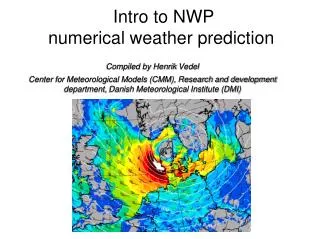
Intro to NWP numerical weather prediction. Compiled by Henrik Vedel Center for Meteorological Models (CMM), Research and development department, Danish Meteorological Institute (DMI). Weather Prediction by Numerical Process. Lewis Fry Richardson, Cambridge University Press, 1922.

E N D
Intro to NWPnumerical weather prediction Compiled by Henrik Vedel Center for Meteorological Models (CMM), Research and development department,Danish Meteorological Institute (DMI)
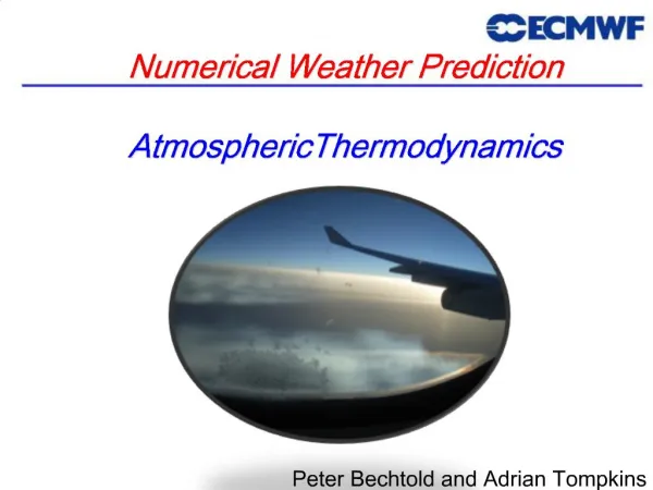
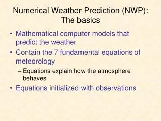
Weather Prediction by Numerical Process Lewis Fry Richardson, Cambridge University Press, 1922 Fundamental equations • Newton's second law • Conservation of mass • Equation of state for ideal gases • Conservation of energy • Conservation of water mass • Effects of radiation, condensation, turbulence, surface friction, lower boundary conditions, etc. • Discretization and solution by finite differences
Kopieret fra ”Atmospheric Data Analysis”, R. Daley, Cambridge Univ. Press
Richardsonestimated 64000 peoplewouldbenecessary for doing global NWP in a ”forecastfactory”. For variousreasons his test, for part of Europe, failed, with huge deviations betweenforecast and observations.
In 1950 NWP was done again, for the US using a real computer, takingabout 24 h to make a 24 h forecast. • Due to more and better observations, faster computer, and better model physics, this time with success. • One reason for the improvement in observations was World War II, whereknowledgeaboutcurrent and future weatherwas in many situation crucial to the planning of military actions.
Fundamental equations • Newton's second law (3 equations for 3D vind) • Conservation of mass (continuity equation) • Equation of state for ideal gases (p, rho, T relation) • Conservation of energy (first law of thermo dynamics) • Conservation of water mass • Effects of radiation, condensation, turbulence, surface friction, lower boundary conditions, etc. • By analysing the equations with atmospheric motions on the Earth in mind simplifications can be made. • Some of these divide NWP models into categories.
Momentum equations See ”An introduction to Dynamical Meteorology”, J. R. Holton, Elsevier Press
Momentum equations See ”An introduction to Dynamical Meteorology”, J. R. Holton, Elsevier Press
Most NWP models arebased on the so-called ”primitive equations”, describing the atmospheric flow under the assumption the vertical flow is muchslowerthan the horisontal, and under the assumption the height of the atmospheresimulated is small compared to the radius of the Earth. • The primitive equationswerefirstwrittendown by Vilhelm Bjerknes, beforeRichardson had his go on a numerical solution.
Example of primitive equations (for a system with pressure as verticalcoordinate, catesian tangent plane in the horisontal, and neglectingcurvature of Earth. Geostrophicwindequations Hydrostatic balance Continuityequation(massconservation), relating horisontal divergence to vertical motions under the hydrostaticapproximation Conservation of energy In addition an equation for conservation of watermass and equation of state Hence the main variables are 2D horisontal wind, temeperature, watervapourcontent, cloudwatercontent and surface pressure.
NWP model coordinate systems • It varies from model to model, in each case care must betaken to ensure proper transformation betweencoordinate systems whentrying to estimate a propertybased on NWP data. • In general: • A NWP model space is spherical or flat (LAM) • Typically g, the graviational acceleration is a fixedconstant. • The height of the model surface is typically the geometricheightwrt. meansealevel (geoid), whendeterminingheightsfurther up, it is typicallythe geopotential heightincrementabove the surface, derived from pressure, density and the hydrostaticapproximation, delta_p = -g rhodelta_z, which is added to the surfaceheight. • The horisontal coordinatesdiffer from model to model, typicallybeingsome type of lat-lon-grid in regional models, to sphericalharmonics and more sofisticatedgrids in global models. Some models are run in gridspace, some in spectralspace.
In most current models the verticalcoordinate is tied to pressure, but is not pressure itself, most commonare, Both have the benefit of being ”terrainfollowing”, the coordinatebeing 1 at the surface, whichsimplifies the equations to solvein the loweratmosphere. The latter has constant pressure surfaces in the upper atmosphere, whichamongotherthingsbenefits the use of importantsatellite data. In some of the newer, non-hydrostatic, models the verticalcoordinate is height
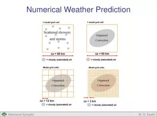
Parametrisations • Operational NWP is mainly done on with horisontal gridsizes of the order 1 to 50 km. • Higher resolution enables more phenomena to resolvedexplicitly by the model. • But at any resolution, many processes occur on too small scale, or aresimplytoocomplex, to beexplicitlyincluded in the model. • Convectiveclouds have sizes of about 1 km, and arecurrently not resolvedproperlyin operational NWP. • Clouds droplet formation occur on molecularscale, is not resolved, and far from understood in detail. Similarly the transfer of solar radiation is related to cloudmicrophisics. Interactions with the ground, relatedsoil type, vegetation type, soilmoistureand resulting evaporation areparametrised.
When the horisontal resolution is increased, to order few km scale, we expect the hydrostatic approximation to become increasingly invalid. Hydrostatic NWP models cannot model the formation of individual convective systems, even the big ones. They are not good at modeling the airflow in regions with strong orography. They do not model gravity waves well at all, which can be of importance sometimes on even larger scales. • (Figure from Arakawa, presentation at workshop on Non-hydrostatic Modelling 8-10 Nov., 2010 ECWMF)
Parameterizations • Land surface • Cloud microphysics • Turbulent diffusion and interactions with surface • Orographic drag • Radiative transfer From J. Knievel
In NWP ”language” processes thatareresolvedareoften referred to as ”dynamics”, whereas processes not explicitlyresolvedare referred to as ”physics”. • The ”physics” is in general ”tuned” for the model to perform the best in the area of interest. For thisreason the NWP models of differentmetoffices or universitiescan perform quitedifferently in differentareas, without it being a real model error . Sometimeseven for the same model, that is just tuneddifferently. • It is important to have this in mind, whenusingresults from different models or from different institutions for a specificarea.
MENU Ingredients of a numericalweatherprediction system Boundary values from external model Observations Computer generated forecasts Data assimilation system provide ”Analysis” (=initial conditions) Numerical weather prediction model Forecasts by forecasters Old model state Combined and done on a very powerfull computer
Examples of HIRLAM (high resolution limitedarea model) run at DMI
Example: HIRLAM S03/SKA details • HIRLAM = High Resolution Limited Area Model • Boundary conditions = ECMWF global model • Horizontal grid resolution = 0.03° (approx 3 km) • Vertical layers = 65 • Grid points = 978 * 818 * 65 • Approximately 8 variables • Forecast length=54h, time step=90s • Runs on 50 nodes (700 cores) using MPI parallelization; asynchronous I/O on 8 cores
Much of the progress in NWP skill is due to faster computers enablingus to increase resolution, improve the data assimilation systems, improve the representation of physical processes. In addition the observing system is graduallyimproving, with more and novel types of observations. • Global models aretypically run 2 – 4 times a day, with forecasts out to about 15 days. • Higher resolution, localarea models (LAMs) are run 4 to 24 times a day, with forecaststypically in the range of 12 hours to severaldays.
Idealised test of N-H versus H NWP model AladinFrom a presentation by Jan MasekSlovak HydroMeteorological Institute (28th EWGLAM meeting 2006)
Findings in idealised tests From Jan Masek
Some examples from DMIMore realistic regarding a focus on real weather phenomenaLess easy to conclude from..
Piteraq i Tasiilaq Feb. 6 1970See Emilie Harmansson, Vejret 126, 2011. Thanks also to Niels Voetmann
Night time radiation results in colder air near surface. In steep orography the denser air slides toward lower levels, accelerating if it continues to be denser. • Hypothesis that N-H NWP is better to model this than hydrostatic NWP because of better handling of vertical dynamics and of orografic forcing. • If air mass moves in an area channeling the air, and into a low pressure area that can “absorb” the air, the wind speed is further increased. • Possibly gravity waves also strengthens the phenomon (similar in foen situations).
NH Arome versus H Aladin, rated by Meteo France forecasters • (from Benard, Meteo France, at workshop 8-10 Nov, 2010, ECMWF)