Parametric Throughput Analysis of Synchronous Data Flow Graphs
310 likes | 519 Vues
Parametric Throughput Analysis of Synchronous Data Flow Graphs. 黃翔. Outline . Abstract Introduction Synchronous Data Flow Graphs(SDFGs) HSDFG Method State-Space Method Divide-and-Conquer Method Experiments Conclusion . Abstract(1/2).

Parametric Throughput Analysis of Synchronous Data Flow Graphs
E N D
Presentation Transcript
Parametric Throughput Analysis of Synchronous Data Flow Graphs 黃翔
Outline • Abstract • Introduction • Synchronous Data Flow Graphs(SDFGs) • HSDFG Method • State-Space Method • Divide-and-Conquer Method • Experiments • Conclusion
Abstract(1/2) • SDFGs have proved to be a very successful tool for modeling, analysis and synthesis of multimedia applications. • One of the most prominent performance constrains of concurrent real-time applications is throughput. • For given actor execution times , throughput can be verified by analyzing the SDFG models of such applications. • Using maximum cycle mean analysis(MCM) or state space analysis.
Abstract(2/2) • In design space exploration(DSE) or runtime reconfiguration, many fast throughput computations are required for varying actor execution times. • We present methods to compute throughput of an SDFG where actor execution times can be parameters. • We propose three different algorithm for parametric throughput analysis and showing the feasibility of the approach. • The divide and conquer algorithm performs best.
Introduction(1/4) • An SDFG is a graph where nodes are called actors and edges are called channels. • Actors typically model application tasks. • Channels model data communication and control dependencies.
Introduction(2/4) • Throughput analysis is a crucial indicator of performance used both at design time(DSE) and runtime(RM). • In DSE many different settings of the system are explored, which leads to many throughput calculations. • At runtime, prediction of throughput is required for proper assignment of resources to applications. • In both cases, throughput calculations need to be as fast as possible with very strict time and resource requirement for runtime applications.
Introduction(3/4) • The execution times of actors are assumed to be fixed numbers in all of the proposed methods. • Any change in the execution time leads to a re-computation of the throughput. • However, calculating the throughput is expensive in many cases, and has exponential time complexity in the worst case. • The worst case execution times of tasks are assigned to actors as their execution times.
Introduction(4/4) • We consider parametric SDFGs, a generalization of SDFGs where can have parameters as their execution times. • We study three algorithms to calculate the throughput of a parametric SDFG. • HSDFG • State-Space Method • Divide-and-Conquer Method
SDFGs(1/4) • Tasks are modeled as actors and channels represent data dependencies. • The execution of an actor is referred to as a firing, the data items communicated between actors are modeled by tokens, and the amounts of tokens produced and consumed in a firing are referred to as rates. • An actor a is tuple (In, Out, ) • Ports of input ports (In(a)) • Ports of output ports (Out(a)) • representing the execution time of
SDFGs(2/4) • When an actor a start its firing, it removes tokens from all In(a). • The firing then continues for time and when it ends, it produces tokens on every Out(a). • An SDFG with all port rates equal to one is called a Homogenous Synchronous Data Flow Graph (HSDFG).
SDFGs(3/4) • The throughput Th(a) of an actor a of an SDFG is defined as the average number of firings of a per time unit in the self-timed execution. • Self-timed execution : firing every actor as soon as it gets enabled. • A parametric SDFG is an SDFG with at least one actor with a parameter as its execution time. • The set of values that the parameters can take, is called the parameter space of the graph.
SDFGs(4/4) • Existing methods of calculating throughput for SDFGs are not directly applicable to parametric SDFGs. • The efficient MCM analysis algorithms which work on HSDFGs cannot be applied on parametric SDFGs. • The conversion of SDFG to HSDFG can easily be adapted though. • However, this conversion may lead to an exponential explosion in the size of the SDFG. • Also, the state-space method cannot be directly used for parametric throughput analysis, but it can be generalized.
HSDFG Method(1/4) • The cycle mean of a cycle of an HSDFG is defined as the total execution time of the cycle over the number of token in that cycle. • The example in fig.1 is already an HSDFG, so no conversion is needed. • This graph has three simple cycles (a,a), (b,b) and (a,b,a) with 1,1 and 3 tokens respectively. • If we assume that the execution times of a and b are given by parameters p and q, the cycle mean expressions are p, q and (p+q)/3 .
HSDFG Method(2/4) • If cycle c has cycle mean expression , then its cycle mean, , for each point in the parameter space can be calculated by . • Ex: • Any expression that has the maximum cycle mean for some point is called a maximum cycle mean expression (mcme). • Any mcme that has the maximum cycle mean value for some point for which no other mcme has the maximum value is a dominating mcme. • The other cycle mean expressions, including the other mcmes, are called redundant expressions.
HSDFG Method(3/4) • The throughput of an SDFG is equal to the inverse of the maximum cycle mean(MCM) of the equivalent HSDFG. • Throughput analysis for a parametric SDFG can be done by finding its DCMS. • Given an HSDFG, the dominating cycle mean set (DCMS) is the set of dominating mcmes. • This minimum set can be obtained from the set of all expressions by removing all redundant expressions. • An expression is redundant if all of its coefficients are less than or equal to those of another expression.
HSDFG Method(4/4) • We see that (p + q)/3 is redundant. • This follows from the infeasible linear system.(Ref.4) • Therefore, DCMS(G)= {p , q}. • Algorithm
State-Space Method(1/7) • State-space-based throughput calculation for SDFGs avoids the conversion to HSDFGs. • The state of SDFG is a tuple • associates with each channel the amount of tokens present in that channel in that state. • associates with each actor a representing the remaining times of different active firings of a.
State-Space Method(2/7) • In fig.1, the initial state is ((1,1,1,2),({},{})). • The first vector shows the token distribution of channels, starting from self-loop channel of a and continuing counterclockwise. • The second vector is the vector of multi-set of the remaining execution times of a and b. • Initially, both multi-set are empty.
State-Space Method(3/7) • Since the relations between parameters are not known, we can not always be sure which firing finishes first. • The parametric state space of with execution times p and q for actors a and b is given in fig.2.
State-Space Method(4/7) • After starting firings of a and b, changes to ({p},{q}). • We split the parameter space into two exclusive parts with p<q and p>q. • From the periodic phase, we can compute the throughput. • The length of the period is (p-q)+q=p and during the period only one firing of actors a and b occurs. • Therefore, the throughput is 1/p if p>q. • The case 2p<q gets period in a few steps with throughput 1/q. • All subsequent branches have the same throughput 1/q.
State-Space Method(5/7) • Since our final goal is finding MCM and since MCM is continuous, we do not need to consider the case p=q as the cycle means of this part of the parameter space are covered by expressions obtained by both the cases p<q and p>q. • We can conclude that, as before, DCMS( )={p , q} for the whole parameter space. • To make the state space finite, we confine the state space, by considering only integer values for parameters.
State-Space Method(6/7) • Algorithm
State-Space Method(7/7) • If a new branch is explored, the nextState is called and the new state n is created. • The search for the recurrent state only occurs in nBList. • If is feasible and n is non-branching, then the algorithm checks whether the state is recurrent. • If the state is recurrent, the algorithm calculates the cycle mean expressions, by calling calcCMExp. • The obtained expression, which is always a dominating mcme, is stored in DCMS. • If is not infeasible but contains no integer solutions, some integer solution may still exist on the border of
Divide-and-Conquer Method(1/4) • This algorithm finds the mcmes of all points in the region including integer solutions on the border of . • If for every corner point of an arbitrary polyhedron of the parameter space, for some mcme then for every point in that region • The parameter space is composed of throughput regions. • Fig.3 shows two throughput regions.
Divide-and-Conquer Method(2/4) • By comparing the evaluation of for every vertex of convex polyhedron C and actual maximum cycle mean value, we can detect whether C is a subset of a single throughput region. • This ideal can be used in a divide-and-conquer method if we add a partitioning strategy. • Partitioning continues till all the created regions have a single mcme. • All obtained mcmes together form the DCMS.
Divide-and-Conquer Method(3/4) • Algorithm
Divide-and-Conquer Method(4/4) • Since MCM is continuous , the mcmes of two neighboring regions are valid for all points on the border. e.g. • We address this plane as the splitting plane. • A randomly selected point from the parameter space has only one mcme with probability one. • All the cycle mean values of all the vertices of convex region(CR) are checked for the validity of the mcme obtained for a random point in the interior of CR. • In case the mcme of is not valid for a vertex , then the splitting plane obtained from mcmes of and splits CR .
Experiments (1/2) • We have evaluated the execution times of our algorithms using SDFG models of 7 real applications.
Experiments (2/2) • We only compared the Divide & Conquer and coverStateSpace algorithm. • The reason is that the HSDFG method works on the HSDFGs, the algorithm takes generally too long. • The results show that a design-time parametric throughput analysis is feasible.
Conclusion • We have extended throughput analysis of SDFGs to parametric SDFGs so that actors can have parameters as their execution times. • We adapted existing methods for computing throughput to parametric SDFGs and proposed a new, faster, algorithm.
