Neural Networks
Neural Networks. Tuomas Sandholm Carnegie Mellon University Computer Science Department. How the brain works. Synaptic connections exhibit long-term changes in the connection strengths based on patterns seen. Comparing brains with digital computers. Parallelism Graceful degradation

Neural Networks
E N D
Presentation Transcript
Neural Networks Tuomas Sandholm Carnegie Mellon University Computer Science Department
How the brain works Synaptic connections exhibit long-term changes in the connection strengths based on patterns seen
Comparing brains with digital computers Parallelism Graceful degradation Inductive learning
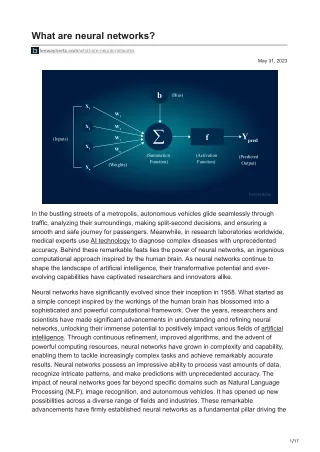
ANN (software/hardware, synchronous/asynchronous) Notation
Activation Functions Where W0,i = t and a0= -1 fixed
W=1 W=1 W= -1 t=-0.5 t=1.5 t=0.5 W=1 W=1 Boolean gates can be simulated by units with a step function AND OR NOT g is a step function
Topologies Feed-forward vs. recurrent Recurrent networks have state (activations from previous time steps have to be remembered): Short-term memory.
Hopfield network • Bidirectional symmetric (Wi,j = Wj,i) connections • g is the sign function • All units are both input and output units • Activations are 1 • “Associative memory” • After training on a set of examples, a new stimulus will cause the network to settle into an activation pattern corresponding to the example in the training set that most closely resemble the new stimulus. • E.g. parts of photograph • Thrm. Can reliably store 0.138 #units training examples
Boltzman machine • Symmetric weights • Each output is 0 or 1 • Includes units that are neither input units nor output units • Stochastic g, i.e. some probability (as a fn of ini) that g=1 • State transitions that resemble simulated annealing. Approximates the configuration that best meets the training set.
Learning in ANNs is the process of tuning the weights Form of nonlinear regression.
ANN topology Representation capability vs. overfitting risk. A feed-forward net with one hidden layer can approximate any continuous fn of the inputs. With 2 hidden layers it can approximate any fn at all. The #units needed in each layer may grow exponentially Learning the topology Hill-climbing vs. genetic algorithms vs. … Removing vs. adding (nodes/connections). Compare candidates via cross-validation.
Perceptrons Implementable with one output unit Decision tree requires O(2n) nodes Majority fn
Representation capability of a perceptron Every input can only affect the output in one direction independent of other inputs. E.g. unable to represent WillWait in the restaurant example. Perceptrons can only represent linearly separable fns. For a given problem, does one know in advance whether it is linearly separable?
Linear separability in 3D Minority Function
Learning linearly separable functions Training examples used over and over! epoch Err = T-O Variant of perceptron learning rule. Thrm. Will learn the linearly separable target fn. (if is not too high) Intuition: gradient descent in a search space with no local optima
Encoding for ANNs E.g. #patrons can be none, some or full Local encoding: None=0.0, Some=0.5, Full=1.0 Distributed encoding: None 1 0 0 Some 0 1 0 Full 0 0 1
Multilayer feedforward networks Structural credit assignment problem Back propagation algorithm (again, Erri=Ti-Oi) Updating between hidden & output units. Updating between input & hidden units: Back propagation of the error
Back propagation (BP) as gradient descent search A way of localizing the computation of the gradient to units.
Observations on BP as gradient descent • Minimize error move in opposite direction of gradient • g needs to be differentiable • Cannot use sign fn or step fn • Use e.g. sigmoid g’=g(1-g) • Gradient taken wrt. one training example at a time
ANN learning curve WillWait problem
Expressiveness of BP 2n/n hidden units needed to represent arbitrary Boolean fns of n inputs. (such a network has O(2n) weights, and we need at least 2n bits to represent a Boolean fn) Thrm. Any continuous fn f:[0,1]nRm Can be implemented in a 3-layer network with 2n+1 hidden units. (activation fns take special form) [Kolmogorov]
Using is fast Training is slow Epoch takes May need exponentially many epochs in #inputs Efficiency of BP
More on BP… Generalization: Good on fns where output varies smoothly with input Sensitivity to noise: Very tolerant of noise Does not give a degree of certainty in the output Transparency: Black box Prior knowledge: Hard to “prime” No convergence guarantees
Summary of representation capabilities (model class) of different supervised learning methods 3-layer feedforward ANN Decision Tree Perceptron K-Nearest neighbor Version space