Spatially Structured Random Effects by Daniel A. Griffith
This presentation summarizes comparisons of spatial structuring methods with selected ecological data for Puerto Rico municipalities, explaining the mechanisms behind community spatial structures and various interpretations of spatial autocorrelation. It also touches on the importance of incorporating spatial community structures into statistical models. The text dives into concepts such as spatial autocorrelation, the Magic Box model, scatterplot trends, and measures like the Moran Coefficient and Geary Ratio.

Spatially Structured Random Effects by Daniel A. Griffith
E N D
Presentation Transcript
Spatially structured random effects by Daniel A. Griffith Ashbel Smith Professor of Geospatial Information Sciences
ABSTRACT Researchers increasingly are employing random effects modeling to analyze data. When data are georeferenced, a random effect term needs to be spatially structured in order to account for spatial autocorrelation. Spatial structuring can be achieved in various ways, including the use of semivariogram,spatial autoregressive, andspatial filter models. SAS implements the semivariogram option for linear mixed models. GeoBUGS implements the spatial autoregressive option for either linear or generalized linear mixed modeling. Recently developed spatial filtering methodology can be used in either case, as well as with the SAS generalized linear mix model procedure, and furnishes one means of estimating space-time mixed models. This presentation summarizes comparisons of these three forms of spatial structuring, illustrating implementations with selected ecological data for the municipalities of Puerto Rico.
Spatial structures in communities indicate that some process hasbeen at work to create them. Two families of mechanisms cangenerate spatial structures in communities: • Autocorrelation model: the spatial structures are generated by thespecies assemblage themselves (response variables). • Induced spatial dependence model: forcing (explanatory) variablesare responsible for the spatial structures found in the speciesassemblage. They represent environmental or biotic control of thespecies assemblages, or historical dynamics To understand the mechanisms that generate these structures, we needto explicitly incorporate the spatial community structures, at all scales, into the statistical model. From Legendre Spatial autocorrelation (SA) is technically defined as the dependence, due to geographic proximity, present in the residuals of a [regression-type] model of a response variable y whicht akes into account all deterministic effects due to forcing variables.
Spatial autocorrelation can be interpreted in different ways As a spatial process mechanism – the cartoon As a diagnostic tool– the Cliff-Ord Eire example (the model specification should be nonlinear) As a nuisance parameter – eliminating spatial dependency to avoid statistical complications As a spatial spillover effect – georeferencing of pediatric lead poisoning cases in Syracuse, NY As an outcome of areal unit demarcation–the modifiable areal unit problem (MAUP) As redundant information – spatial sampling; map interpolation As map pattern – spatial filtering (to be discussed in this course) As a missing variables indicator/surrogate – a possible implication of spatial filtering As self-correlation – what is discussed next
The SASIM game http://www.nku.edu/~longa/cgi-bin/cgi-tcl-examples/generic/SA/SA.cgi
Measures of spatial autocorrelation MC: Moran Coefficient;GR: Geary Ratio;semivariogram Spherical Exponential Bessel function (1st order, 2nd kind)
Georeferenced data scatterplots • The horizontal axis is the measurement scale for some attribute variable • The vertical axis is the measurement scale for neighboring values (topological distance-based) of the same attribute variable OR • The horizontal axis is (usually) Euclidean distance between geocoded locations • The vertical axis is the measurement scale for geographic variability
Describing a scatterplot trend positive relationship: High Y with High X & Medium Y with Medium X & Low Y with Low X negative relationship: High Y with Low X & Medium Y with Medium X & Low Y with High X
Description of the Moran scatterplot 2002 population density Positive spatial autocorrelation - high values tend to be surrounded by nearby high values - intermediate values tend to be surrounded by nearby intermediate values - low values tend to be surrounded by nearby low values MC = 0.49 GR = 0.58
Description of the Moran scatterplot competition for space Negative spatial autocorrelation - high values tend to be surrounded by nearby low values - intermediate values tend to be surrounded by nearby intermediate values - low values tend to be surrounded by nearby high values MC = -0.16 sMC = 0.075 GR = 1.04
Graphical portrayals of spatial autocorrelation latent in transformed As data
Constructing eigenfunctions for filtering spatial autocorrelation out of georeferenced variables: Moran Coefficient = (n/1T C1)x YT(I – 11T/n)C (I – 11T/n)Y/ YT(I – 11T/n)Y the eigenfunctions come from (I – 11T/n)C (I – 11T/n)
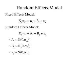
Random effects model is a random observation effect (differences among individual observational units) is a time-varying residual error (links to change over time) The composite error term is the sum of the two.
Random effects model: normally distributed intercept term • ~ N(0, ) and uncorrelated with covariates • supports inference beyond the nonrandom sample analyzed • simplest is where intercept is allowed to vary across areal units (repeated observations are individual time series) • The random effect variable is integrated out (with numerical methods) of the likelihood fcn • accounts for missing variables & within unit correlation (commonality across time periods)
Spatial structuring of random effects • CAR: conditional autoregressive model • ICAR: improper conditional autoregressive model (spatial autocorrelation set to 1,and a spatially structured and a spatially unstructured variance component is estimated)─should be specified as a convolution prior (spatially structured & unstructured random effects) • SF: spatial filter identified with a frequentist GLM
Impact of sample size • prior • distribution As the sample size increases, a prior distri-bution has less and less impact on results; BUT • likelihood • distribution • effective • sample size • for spatially • autocorrelated • data
What is BUGS? Bayesian inference Using Gibbs Sampling • is a piece of computer software for the Bayesian analysis of complex statistical models using Markov chain Monte Carlo (MCMC) methods. • It grew from a statistical research project at the MRC BIOSTATISTICAL UNIT in Cambridge, but now is developed jointly with the Imperial College School of Medicine at St Mary’s, London.
Classic BUGS • WinBUGS (Windows Version) • BUGS • GeoBUGS (spatial models) • PKBUGS (pharmokinetic modeling) • The Classic BUGS program uses text-based model description and a command-line interface, and versions are available for major computer platforms (e.g., Sparc, Dos). However, it is not being further developed.
What is WinBUGS? • WinBUGS, a windows program with an option of a graphical user interface, the standard ‘point-and-click’ windows interface, and on-line monitoring and convergence diagnostics. It also supports Batch-mode running (version 1.4). • GeoBUGS, an add-on to WinBUGS that fits spatial models and produces a range of maps as output. • PKBUGS, an efficient and user-friendly interface for specifying complex population pharmacokinetic and pharmacodynamic (PK/PD) models within the WinBUGS software.
What is GeoBUGS? • Available via http://www.mrc-bsu.cam.ac.uk/ bugs/winbugs/geobugs.shtml • Bayesian inference is used to spatially smooth the standardized incidence ratios using Markov chain Monte Carlo (MCMC) methods. GeoBUGS implements models for data that are collected within discrete regions (not at the individual level), and smoothing is done based on Markov random field models for the neighborhood structure of the regions relative to each other.
What is MCMC? MCMC is used to simulate from some distribution p known only up to a constant factor, C: pi = Cqi where qi is known but C is unknown and too horrible to calculate. MCMC begins with conditional (marginal) distributions, and MCMC sampling outputs a sample of parameters drawn from their posterior (joint) distribution.
The geographic distribution of elevation across the island of Puerto Rico From a USGS DEM containing 87,358,136 points. Darkness of gray scale is directly proportional to elevation.
SAS PROC MIXED summary results for a quadratic gradient LMM: LN( + 17.5)
ICAR The average random effects term example MCMC chain from a WinBUGS run spatial filter (SF)
spatial filter (SF) WinBUGS: geographic distributions of unstructured (left) and spatially structured (right) random effects WinBUGS: ICAR
Comparative parameter estimates for a LMM quadratic gradient description of LN( + 17.5) varure denotes the variance of the unstructured random effects varssre denotes the variance of the spatially structured random effects
SAS SF binomial GLMM random effects WinBUGS SF WinBUGS ICAR
Graphical diagnostics of residuals for the GLMM estimated with SAS
Scatterplot of the SAS and mean WinBUGS estimated spatially structured random effects terms
Individual GLMM estimation results for each Puerto Rican sugar cane crop year
random effect (re) re + ss: 1965/66 Space-time data: preliminaries re + ss: 1967/68 Random effects term is constant across time; spatial structuring changes over time re + ss: 1966/67
Space-time GLMM: Puerto Rican sugar cane crop years 1965/66-1967/68 when all fixed effects are year-specific
Discussion & Implications All three common specifications of spatial structuring—semivariogram, spatial autoregressive and SF models—for a random effect term in mixed statistical models perform in an equivalent fashion. Matching Bayesian model priors with their implicit frequentist counterparts yields estimation results from both approaches that are essentially the same. making use of spatially structured random effects tends to furnish an alternative to quasi-likelihood estimation techniques for GLMMs
Semivariogram models offer a geostatistical theoretical basis and have been implemented in SAS for LMMs. • A spatial statistics practitioner with the necessary computer programming skills can employ WinBUGS in order to utilize them with GLMMs. • Spatial autoregressive modeling offers a theoretical basis for spatial structuring, and is available in GeoBUGS. • This would be very difficult to trick SAS into doing. • Spatial filtering, which can be derived from spatial autoregressive model specifications, • tends to be more exploratory in nature (being akin to principal components analysis) • can be implemented in either SAS or WinBUGS for either LMMs or GLMMs, and • can be easily extended to space-time datasets with either of these software packages.
Illustrative Puerto Rico sugar cane examples tend to have a random effect term that virtually equates to the corresponding LMM/GLMM residual variate. • This is not always the case, as is highlighted by the extension of a GLMM specification to a space-time sugar cane dataset. • All of the estimated random effects terms for the various Puerto Rico examples tend to be non-normal.
once a random effect term has been estimated with a frequentist approach, using it when calculating a deviance statistic allows its number of degrees of freedom to be approximated for GLMMs. • Although n values are estimated, because they are correlated, the resulting number of degrees of freedom is less than n. • This particular finding should help spatial statistics practitioners better understand the cost of employing a statistical mixed model.
A df aside: future research • Spiegelhalter et al. (2002) address the df problem for complex hierarchical models in which the number of parameters is not clearly defined because, for instance, of the presence of random effects. • An information-theoretic argument is used to approximate the effective number of parameters in a model, equivalent to the trace of the product of the Fisher information and the posterior covariance matrices. • this particular approximation is equivalent to the trace of the ‘hat’ matrix for linear models with a normally distributed error term.


