Random Effects Model
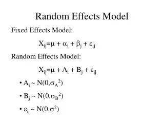
Random Effects Model. Fixed Effects Model: X ij = + i + j + ij Random Effects Model: X ij = + A i + B j + ij A i ~ N(0, A 2 ) B j ~ N(0, B 2 ) ij ~ N(0, 2 ). Random Effects Model Cont’d. Hypotheses:

Random Effects Model
E N D
Presentation Transcript
Random Effects Model • Fixed Effects Model: • Xij= + i + j + ij • Random Effects Model: • Xij= + Ai + Bj + ij • Ai ~ N(0,A2) • Bj ~ N(0,B2) • ij ~ N(0,2)
Random Effects Model Cont’d • Hypotheses: • HoA: A2 = 0, HoB:B2 = 0 • HaA:A2 > 0, HaB: B2 > 0 • E(MSA) = 2+JA2 • E(MSB) = 2+JB2 • E(MSE) = 2 fA= E(MSA) / E(MSE) fB= E(MSB) / E(MSE)
Mixed Effects Model • Xij= + i + Bj + ij • HoA: 1=…=n= 0 , HoB: B2 =0 • HaA: at least one i differs, HaB:B2 > 0 • E(MSA) = 2+(J/I-1)i • E(MSB) = 2+JB2 • E(MSE) = 2 fA= E(MSA) / E(MSE) fB= E(MSB) / E(MSE)
Example – Blocking (Fixed and Random Effects) (11.6,12) A particular county has 3 assessors who determine the value of residential property. To test whether the assessors systematically differ, 5 houses are selected and each assessor is asked to determine their value. Let factor A denote the assessor and factor B denote the the houses. We compute SSA=11.7, SSB=113.5, and SSE = 25.6
Example Cont’d Suppose that the 6 houses in the previous example had been selected at random from among those of a certain age and size. It follows that factor B is random rather than fixed
Two-Factor ANOVA, Kij>1(11.2) • When Kij>1, an estimator of the the variance 2 (MSE) of may be obtained without assuming additivity. • This allows for our model to include an interaction parameter • Assume that Kij = K >1 for all i,j
The Model • Let : • ij = The true average response when factor A is at level i and factor B at level j • = (j j ij)/IJ = The true grand mean • i·= (j ij)/J = The expected response of factor A at level i averaged over factor B • ·j= (i ij)/I = The expected response of factor B at level j averaged over factor A
The Model Cont’d • i = i·- = The effect of factor A at level i (main effects for factor A) • j = ·j- = The effect of factor B at level j (main effects for factor B) • ij = ij – ( + i + j ) = interaction effect of factor A at level i and factor B at level j (interaction parameters) • ij = + i + j + ij
The Model Cont’d Xijk= + i + Bj + ij + ijk , ijk ~ N(0,2) Hypotheses: HoAB: ij = 0, HaAB = at least one ij 0 HaA: 1=…=n= 0 , HaA:at least one i 0 HaB: 1=…=n= 0 , HaB:at least one i 0
The Test • Test the no-interaction hypothesis HoAB first • If HoAB is not rejected • Test the other hypothesis HoA and HoB • If HoAB is rejected • Do not test the other hypothesis HoA and HoB • Construct an interaction plot to visualize how the factors interact
The Test Cont’d Assume that we reject HoAB and then go on to test HoA and HoB. Suppose that HoA is rejected. The resulting model would be ij = + j + ij which does not have a clear interpretation. In other words, an insignificant main effect has little meaning in the presence of a significant interaction effect.
The Test Cont’d • E(MSA) = 2+(JK/I-1)i2 • E(MSB) = 2+(IK/J-1)i2 • E(MSAB) = 2+[K/((I-1)(J-1))]ij2 • E(MSE) = 2 fA= E(MSA) / E(MSE) fB= E(MSB) / E(MSE) fAB= E(MSAB) / E(MSE)
Example (11.19) The accompanying data gives observations of the total acidity of coal samples of three different types, with determinations made using three different concentrations of NaOH. Assuming fixed effects, construct an ANOVA table and test for the presence of interactions and main effects at los 0.01