The Mixed, Random Effects Model for Continuous Outcomes
420 likes | 586 Vues
The Mixed, Random Effects Model for Continuous Outcomes. References Analysis of Longitudinal Data by Diggle, Liang and Zeger . Laird and Ware, 1982, Biometrics 38: 963-974. What’s being “Mixed”?. A mixed model has two types of effects, fixed and random .

The Mixed, Random Effects Model for Continuous Outcomes
E N D
Presentation Transcript
The Mixed, Random Effects Model for Continuous Outcomes References Analysis of Longitudinal Data by Diggle, Liang and Zeger. Laird and Ware, 1982, Biometrics 38: 963-974.
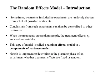
What’s being “Mixed”? • A mixed model has two types of effects, fixed and random. • A fixed effect means that all levels of the variable are contained in the data and the effect is universal to all in the target population. • A random effect means that the levels (effects) of the variable comprise random samples of the levels (effects) in the target population. • Consider a treatment effect. Fixed, Random, Both?
Why Use mixed models? • The model implies correlation between measurements on the same subject (note previous examples and assignments). • Permits one to specify a rich set of correlation models and allows for heteroskedascity. • It allows different subjects to have different responses to a treatment, risk variable, etc., thus has intuitive appeal. • Estimation can return both fixed effects and estimate the variability of different factors in your data (e.g., within-subject, between subject, clinic,etc.).
Estimation of coefficients using mixed models • As we’ve showed in class and homework, random effects models imply certain variance-covariance structures. • For instance, a simple random effects model results in equal correlation (exchangeable or compound symmetry) among all observations measured on the same subject. • We know that if the variance-covariance matrix (V) is known, then the most efficient estimate of the coefficients is weighted-least squares: where W = V-1. • W
Estimation of coefficients using mixed models, cont. • The Mixed Model procedure works by: • Converting the random effects model into its implied variance-covariance matrix, V, • starting with the independent model (OLS) it gets residuals and then estimates V based on this model, • creates weight matrix as , • does weighted least squares and gets residuals, • repeats until convergence. • The SE’s the procedure return come from:
Danger of using mixed models for continuous outcomes • When deriving the inference on coefficients, the estimating procedure assumes that the variance-covariance model of the outcome implied by the model IS CORRECT (i.e., it’s always naïve, not “robust”).
The Simplest Example. • The Model: • E(i)=0, E(eij)=0, E[i eij]=0. • Var(i)= 2. • Var(eij)= 2e . • What are the fixed and random effects in this model?
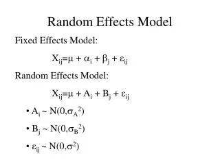
A more complicated example. • The Model: • E(0i)=0, E(1i)=0, E(eij)=0. • Var(0i)= 20, Var(1i)= 21, Var(eij)= 2 • cov(0i, 1i)= 12, cov(0i, eij)=0, cov(1i, eij)=0. • What are the fixed and random effects in this model?
Mixed Model I for Dental Data • First, the Model where xij, is the jth age of ith child, Yij is the distance. • E(0i)=0, E(eij)=0. • Var(0i)= 20, Var(eij)= 2 • cov(0i, eij)=0. • What are the fixed and random effects in this model?
SAS – Dental Model I Code proc mixed data=temp1; class child; model distance = age / s; random int / sub=child s; run; Output Covariance Parameter Estimates Cov Parm Subject Estimate Intercept child 4.472120 Residual 2.0495 2 Fit Statistics -2 Res Log Likelihood 447.0 AIC (smaller is better) 451.0 AICC (smaller is better) 451.1 BIC (smaller is better) 453.6
SAS – Dental Model I, cont. Solution for Fixed Effects Standard Effect Estimate Error DF t Value Pr > |t| Intercept 16.7611 0.8024 26 20.89 <.0001 age 0.6602 0.06161 80 10.72 <.0001 Solution for Random Effects 0i Std Err Effect child Estimate Pred DF t Value Pr > |t| Intercept 1 -2.3759 0.7799 80 -3.05 0.0031 Intercept 2 -0.9180 0.7799 80 -1.18 0.2427 Intercept 3 -0.2451 0.7799 80 -0.31 0.7542 Intercept 4 0.7643 0.7799 80 0.98 0.3301 Intercept 5 -1.2544 0.7799 80 -1.61 0.1117 Intercept 6 -2.6002 0.7799 80 -3.33 0.0013 Intercept 7 -0.9180 0.7799 80 -1.18 0.2427 Intercept 8 -0.5815 0.7799 80 -0.75 0.4581 Intercept 9 -2.6002 0.7799 80 -3.33 0.0013
STATA – XTREG . xtreg distance age, i(child) re Random-effects GLS regression Number of obs = 108 Group variable (i) : child Number of groups = 27 R-sq: within = 0.5894 Obs per group: min = 4 between = . avg = 4.0 overall = 0.2565 max = 4 Random effects u_i ~ Gaussian Wald chi2(1) = 114.84 corr(u_i, X) = 0 (assumed) Prob > chi2 = 0.0000 ------------------------------------------------------------------------------ distance | Coef. Std. Err. z P>|z| [95% Conf. Interval] -------------+---------------------------------------------------------------- age | .6601852 .0616059 10.72 0.000 .5394398 .7809306 _cons | 16.76111 .8023952 20.89 0.000 15.18845 18.33378 -------------+---------------------------------------------------------------- 0 sigma_u | 2.1147235 sigma_e | 1.4315921 rho | .68573911 (fraction of variance due to u_i) ------------------------------------------------------------------------------
STATA – XTGEE non-robust . xtgee distance age, i(child) cor(exc) Iteration 1: tolerance = 4.001e-16 GEE population-averaged model Number of obs = 108 Group variable: child Number of groups = 27 Link: identity Obs per group: min = 4 Family: Gaussian avg = 4.0 Correlation: exchangeable max = 4 Wald chi2(1) = 116.27 Scale parameter: 6.317927 Prob > chi2 = 0.0000 ------------------------------------------------------------------------------ distance | Coef. Std. Err. z P>|z| [95% Conf. Interval] -------------+---------------------------------------------------------------- age | .6601852 .0612245 10.78 0.000 .5401875 .7801829 _cons | 16.76111 .7945636 21.09 0.000 15.2038 18.31843 ------------------------------------------------------------------------------
STATA – XTGEE robust for comparison Iteration 1: tolerance = 4.001e-16 GEE population-averaged model Number of obs = 108 Group variable: child Number of groups = 27 Link: identity Obs per group: min = 4 Family: Gaussian avg = 4.0 Correlation: exchangeable max = 4 Wald chi2(1) = 85.85 Scale parameter: 6.317927 Prob > chi2 = 0.0000 (standard errors adjusted for clustering on child) ------------------------------------------------------------------------------ | Semi-robust distance | Coef. Std. Err. z P>|z| [95% Conf. Interval] -------------+---------------------------------------------------------------- age | .6601852 .0712533 9.27 0.000 .5205313 .799839 _cons | 16.76111 .7752462 21.62 0.000 15.24166 18.28057 ------------------------------------------------------------------------------ Note, that the robust SE’s are not the same as the non-robust
Mixed Model II for Dental Data • The Model (called a random coefficients model) • E(0i)=0, E(1i)=0, E(eij)=0. • Var(0i)= 20, Var(1i)= 21, Var(eij)= 2 • cov(0i, 1i)= 12, cov(0i, eij)=0, cov(1i, eij)=0.
SAS – Dental Model II Code proc mixed data=temp1; class child; model distance = age / s; random int age / sub=child s; run; Output Cov Parm Subject Estimate Intercept child 1.9211 20 age child 0.02228 21 Residual 1.8787 2 Fit Statistics -2 Res Log Likelihood 443.3 AIC (smaller is better) 449.3 AICC (smaller is better) 449.5 BIC (smaller is better) 453.2
SAS – Dental Model II, cont. Solution for Fixed Effects Standard Effect Estimate Error DF t Value Pr > |t| Intercept 16.7611 0.7138 26 23.48 <.0001 age 0.6602 0.06561 26 10.06 <.0001 Solution for Random Effects 0i, 1i Std Err Effect child Estimate Pred DF t Value Pr > |t| Intercept 1 -0.8605 1.0693 54 -0.80 0.4245 age 1 -0.1434 0.09948 54 -1.44 0.1553 Intercept 2 -0.5541 1.0693 54 -0.52 0.6064 age 2 -0.03033 0.09948 54 -0.30 0.7617 Intercept 3 -0.2831 1.0693 54 -0.26 0.7922 age 3 0.007197 0.09948 54 0.07 0.9426 Intercept 4 0.5223 1.0693 54 0.49 0.6272 age 4 0.01835 0.09948 54 0.18 0.8543 Intercept 5 -0.2463 1.0693 54 -0.23 0.8187 age 5 -0.09924 0.09948 54 -1.00 0.3230
Strength Data • Subjects randomized to one of 3 treatments • No training (tx=1) • Weight training with light weights and high repetition (tx=2) • Weight training with heavy weights and low repetition (tx=3) • Subjects were followed for 7 weeks and a measure of muscle strength was recorded each week. • The questions of interest are • Does weight training have any impact on strength? • Is there a difference between tx 2 and 3? • Which training program works quickest to increase strength?
Strength Data id tx y time 1. 1 1 85 1 2. 1 1 85 2 3. 1 1 86 3 4. 1 1 85 4 5. 1 1 87 5 6. 1 1 86 6 7. 1 1 . 7 8. 2 1 80 1 9. 2 1 79 2 10. 2 1 . 3 11. 2 1 78 4 12. 2 1 78 5 13. 2 1 79 6 14. 2 1 . 7
Mixed Model I for Strength Data • First, the Model (xij, time of ijth measurement, Txi is the treatment assignment for ith person). • E(0i)=0, E(eij)=0. • Var(0i)= 20, Var(eij)= 2 • cov(0i, eij)=0. • What are the fixed and random effects in this model?
SAS – Strength Model I Code proc mixed data=temp1; class id tx; model y = time tx tx*time / s; random int / sub=id s; run; Output Cov Parm Subject Estimate Intercept id 9.3645 20 Residual 1.1668 2 Fit Statistics -2 Res Log Likelihood 1336.2 AIC (smaller is better) 1340.2 AICC (smaller is better) 1340.2 BIC (smaller is better) 1344.2
SAS Strength Model I, cont. Solution for Fixed Effects Standard Effect tx Estimate Error DF t Value Pr > |t| Intercept 81.0184 0.6986 54 115.98 <.0001 time 0.3039 0.04851 310 6.27 <.0001 tx 1 -0.9567 0.9998 310 -0.96 0.3394 tx 2 -1.1488 1.0618 310 -1.08 0.2801 tx 3 0 . . . . time*tx 1 -0.3732 0.06837 310 -5.46 <.0001 time*tx 2 -0.06113 0.07178 310 -0.85 0.3951 time*tx 3 0 . . . . Solution for Random Effects 0i Std Err Effect id Estimate Pred DF t Value Pr > |t| Intercept 1 5.7287 0.8055 310 7.11 <.0001 Intercept 2 -0.9875 0.8259 310 -1.20 0.2328 Intercept 3 -2.8760 0.7902 310 -3.64 0.0003 Intercept 4 4.2823 0.7902 310 5.42 <.0001 Intercept 5 0.07153 0.7902 310 0.09 0.9279 Intercept 6 -2.8760 0.7902 310 -3.64 0.0003 Intercept 7 -0.2092 0.7902 310 -0.26 0.7914
ANOVA table from SAS Strength Model I Type 3 Tests of Fixed Effects Num Den Effect DF DF F Value Pr > F time 1 310 30.49 <.0001 tx 2 310 0.72 0.4880 time*tx 2 310 16.93 <.0001
STATA for Strength Data - XTREG . gen tx1 = tx==1 . gen tx2 = tx==2 . gen tx1time = tx1*time . gen tx2time = tx2*time . xi: xtreg y tx1 tx2 time tx1time tx2time, i(id) re mle Random-effects ML regression Number of obs = 370 Group variable (i) : id Number of groups = 57 Random effects u_i ~ Gaussian Obs per group: min = 5 avg = 6.5 max = 7 LR chi2(5) = 63.37 Log likelihood = -663.52557 Prob > chi2 = 0.0000 ------------------------------------------------------------------------------ y | Coef. Std. Err. z P>|z| [95% Conf. Interval] -------------+---------------------------------------------------------------- tx1 | -.9568027 .9747104 -0.98 0.326 -2.8672 .9535947 tx2 | -1.148717 1.035118 -1.11 0.267 -3.177512 .8800772 time | .3038536 .048275 6.29 0.000 .2092364 .3984709 tx1time | -.3731916 .0680398 -5.48 0.000 -.5065472 -.2398361 tx2time | -.0611408 .0714338 -0.86 0.392 -.2011484 .0788669 _cons | 81.0185 .6810685 118.96 0.000 79.68363 82.35337 -------------+---------------------------------------------------------------- /sigma_u | 2.97753 .2846527 10.46 0.000 2.419621 3.535439 /sigma_e | 1.074968 .0429662 25.02 0.000 .9907563 1.159181 -------------+---------------------------------------------------------------- rho | .8846892 .0212074 .8376945 .9210974 ------------------------------------------------------------------------------ Likelihood ratio test of sigma_u=0: chibar2(01)= 571.45 Prob>=chibar2 = 0.000
STATA for Strength Data, cont. • Test of no treatment effect, H0: b4 = b5 = 0. . test tx1time tx2time ( 1) [y]tx1time = 0.0 ( 2) [y]tx2time = 0.0 chi2( 2) = 34.17 Prob > chi2 = 0.0000
Equivalent STATA for Strength Data, XTGEE with exchangeable . . xtgee y tx1 tx2 time tx1time tx2time, i(id) cor(exc) Iteration 1: tolerance = .04128019 Iteration 2: tolerance = .00001468 Iteration 3: tolerance = 2.476e-09 GEE population-averaged model Number of obs = 370 Group variable: id Number of groups = 57 Link: identity Obs per group: min = 5 Family: Gaussian avg = 6.5 Correlation: exchangeable max = 7 Wald chi2(5) = 64.83 Scale parameter: 9.918406 Prob > chi2 = 0.0000 ------------------------------------------------------------------------------ y | Coef. Std. Err. z P>|z| [95% Conf. Interval] -------------+---------------------------------------------------------------- tx1 | -.956994 .9684046 -0.99 0.323 -2.855032 .9410442 tx2 | -1.148591 1.028411 -1.12 0.264 -3.164239 .8670575 time | .3037201 .0501318 6.06 0.000 .2054634 .4019767 tx1time | -.3730803 .0706584 -5.28 0.000 -.5115681 -.2345924 tx2time | -.0611578 .0741834 -0.82 0.410 -.2065545 .0842389 _cons | 81.0188 .6766896 119.73 0.000 79.69251 82.34509 ------------------------------------------------------------------------------ .
Equivalent STATA for Strength Data, XTGEE with exchangeable . xtcorr c1 c2 c3 c4 c5 c6 c7 r1 1.0000 r2 0.8743 1.0000 r3 0.8743 0.8743 1.0000 r4 0.8743 0.8743 0.8743 1.0000 r5 0.8743 0.8743 0.8743 0.8743 1.0000 r6 0.8743 0.8743 0.8743 0.8743 0.8743 1.0000 r7 0.8743 0.8743 0.8743 0.8743 0.8743 0.8743 1.0000
Equivalent STATA for Strength Data, XTGEE with exchangeable, robust . xtgee y tx1 tx2 time tx1time tx2time, i(id) cor(exc) robust GEE population-averaged model Number of obs = 370 Group variable: id Number of groups = 57 Link: identity Obs per group: min = 5 Family: Gaussian avg = 6.5 Correlation: exchangeable max = 7 Wald chi2(5) = 33.82 Scale parameter: 9.918406 Prob > chi2 = 0.0000 (standard errors adjusted for clustering on id) ------------------------------------------------------------------------------ | Semi-robust y | Coef. Std. Err. z P>|z| [95% Conf. Interval] -------------+---------------------------------------------------------------- tx1 | -.956994 .9449735 -1.01 0.311 -2.809108 .89512 tx2 | -1.148591 1.057032 -1.09 0.277 -3.220334 .9231534 time | .3037201 .0698707 4.35 0.000 .1667761 .440664 tx1time | -.3730803 .1036701 -3.60 0.000 -.57627 -.1698906 tx2time | -.0611578 .1320877 -0.46 0.643 -.3200449 .1977294 _cons | 81.0188 .7302755 110.94 0.000 79.58749 82.45011 ------------------------------------------------------------------------------
Mixed Model II for Strength Data • The Model: • E(0i)=0, E(1i)=0, E(eij)=0. • Var(0i)= 20, Var(1i)= 21, Var(eij)= 2 • cov(0i, 1i)= 12, cov(0i, eij)=0, cov(1i, eij)=0.
SAS – Strength Model II Code proc mixed data=temp1; class id tx; model y = time tx tx*time / s; random int time / sub=id s; run; Output Covariance Parameter Estimates Cov Parm Subject Estimate Intercept id 8.7247 20 time id 0.1159 21 Residual 0.6676 2 Fit Statistics -2 Res Log Likelihood 1250.0 AIC (smaller is better) 1256.0 AICC (smaller is better) 1256.1 BIC (smaller is better) 1262.1
SAS – Strength Model II, cont. Solution for Fixed Effects Standard Effect tx Estimate Error DF t Value Pr > |t| Intercept 80.9292 0.6635 54 121.98 <.0001 time 0.3368 0.08352 54 4.03 0.0002 tx 1 -0.8779 0.9495 256 -0.92 0.3561 tx 2 -1.0334 1.0083 256 -1.02 0.3064 tx 3 0 . . . . time*tx 1 -0.4010 0.1189 256 -3.37 0.0009 time*tx 2 -0.1018 0.1259 256 -0.81 0.4195 time*tx 3 0 . . . . Solution for Random Effects 0i, 1i Std Err Effect child Estimate Pred DF t Value Pr > |t| Intercept 1 4.6708 0.9232 256 5.06 <.0001 time 1 0.3171 0.1781 256 1.78 0.0762 Intercept 2 -0.4756 0.9438 256 -0.50 0.6148 time 2 -0.1492 0.1789 256 -0.83 0.4049 Intercept 3 -2.3295 0.9002 256 -2.59 0.0102 time 3 -0.1456 0.1551 256 -0.94 0.3488 Intercept 4 3.8359 0.9002 256 4.26 <.0001 time 4 0.1177 0.1551 256 0.76 0.4486 Intercept 5 0.4222 0.9002 256 0.47 0.6395 time 5 -0.09100 0.1551 256 -0.59 0.5578
ANOVA table from SAS Strength Model II Type 3 Tests of Fixed Effects Num Den Effect DF DF F Value Pr > F time 1 54 11.20 0.0015 tx 2 256 0.66 0.5200 time*tx 2 256 6.06 0.0027
Using Splus on Strength Data – Model II > lme.strength.2 <- lme(fixed = y ~ time + tx1 + tx2 + tx1time + tx2time, random = ~ 1 + time | id, data = strength, na.action = na.omit) > summary(lme.strength.2) Linear mixed-effects model fit by REML Data: strength AIC BIC logLik 1269.113 1308.084 -624.5564 Random effects: Formula: ~ 1 + time | id Structure: General positive-definite StdDev Corr (Intercept) 2.9916910 (Inter 0 time 0.3453682 -0.146 1 12 Residual 0.8151103 Fixed effects: y ~ time + tx1 + tx2 + tx1time + tx2time Value Std.Error DF t-value p-value (Intercept) 80.92928 0.671454 310 120.5284 <.0001 time 0.33665 0.084446 310 3.9866 0.0001 tx1 -0.87757 0.960890 54 -0.9133 0.3651 tx2 -1.03163 1.020390 54 -1.0110 0.3165 tx1time -0.40100 0.120222 310 -3.3355 0.0010 tx2time -0.10242 0.127293 310 -0.8046 0.4217
Using Splus on Strength Data – Model I > lme.strength.1 <- lme(fixed = y ~ time + tx1 + tx2 + tx1 * time + tx2 * time, random = ~ 1 | id, data = strength.dat, na.action = na.omit) > summary(lme.strength.1) Linear mixed-effects model fit by REML Data: strength.dat AIC BIC logLik 1352.16 1383.337 -668.08 Random effects: Formula: ~ 1 | id (Intercept) Residual StdDev: 3.060553 1.080153 (0) Fixed effects: y ~ time + tx1 + tx2 + tx1 * time + tx2 * time Value Std.Error DF t-value p-value (Intercept) 81.01837 0.698662 310 115.9621 <.0001 time 0.30391 0.048508 310 6.2652 <.0001 tx1 -0.95672 0.999908 54 -0.9568 0.3429 tx2 -1.14877 1.061883 54 -1.0818 0.2841 tx1:time -0.37324 0.068369 310 -5.4592 <.0001 tx2:time -0.06113 0.071779 310 -0.8517 0.3950
Fixed and Random Effects > lme.strength.2$coefficients $fixed: (Intercept) time tx1 tx2 tx1time tx2time 80.92928 0.3366547 -0.8775729 -1.031627 -0.4009952 -0.1024152 $random: $random$id: (Intercept) time 0i 1i 1 4.7153235 0.30295696 2 -0.4708943 -0.14976759 3 -2.3472132 -0.14065535 4 3.8722475 0.10820261 5 0.4327349 -0.09333664 6 -2.2308728 -0.16995496 7 -1.1228466 0.22724303 8 -3.4205332 -0.29745005 9 -2.7047801 0.47696378 10 -0.9647069 -0.04676567 11 0.3295226 0.14620860 12 -3.1400180 0.09459964
Fixed and Random Effects > lme.strength.1$coefficients $fixed: (Intercept) time 80.36677 0.1531045 $random: $random$id: 0i (Intercept) 1 4.66415489 2 -2.06488079 3 -4.04774444 4 3.10664991 5 -1.10181736 6 -4.04774444 7 -1.38238184 8 -5.73113134 9 -2.05089747 10 -2.21406991 11 -0.26012390 12 -3.90746220 13 1.98439197 14 0.58156955 15 -0.09282822