Download
1 / 6
60 likes | 197 Vues
This analysis focuses on the incorporation of skewed random effects into the AD model, particularly in the context of diet and its relation to heart disease as described in Section 14.2 of Skrondal and Rabe-Hesketh's Generalized Latent Variable Modeling. The study involves 337 middle-aged men, examining the impacts of age and public transport usage on fiber intake and subsequent heart disease risk. The model is set up in R, using advanced statistical techniques such as Laplace approximation and Gauss-Hermite quadrature to estimate the effects of dietary variables while accounting for covariate measurement error.

E N D
Goal • Analyse model in Section 14.2 of Skrondal and Rabe-Hesketh (2004) Generalized Latent Variable Modeling: Multilevel, Longitudinal and Structural Equation Models. Chapman & Hall • Replace normal distribution with a skewed distribution for the random effects.
14.2 Diet and heart disease • Covariate measurement error model • 337 middle aged men (bank, transportation) • At requirement: weigh their food • Repeated measurement for 76 men • Heart disease or not? • Covariates: • age (numeric) • bus (0,1)
Model description • Exposure model (true fiber intake) ηj = γ1·agej+γ2·busj + γ3·age*busj+ ζj, ζj ~ N(0, ψ) • Measured fiber intake (i = 1,2) yij = ηj + α0+(i-1)·α1 + ij , ij ~ N(0, θ) • Disease model(D = 0,1) logit(Dj|ηj) = β0 +β1·agej+β2·busj + β3·age*busj + λ·ηj
Setting up and running the model • Prepare data in R: ”diet.s” • Compiling the model • admb -re diet • Running the model (Laplace approx.) • diet -est • Running the model (Gauss-Hermite appr.) • diet -est -gh 20
Skewed distributions for ζ • Skrondal and Rable-Hesket: • Replace N(0,ψ) distribution for ζj by non-parametric distribution (Fig. 14.2) • Skewed distribution for ζj ζj = [a·uj + (1-a)[exp(uj)-exp(0.5)]/c1]/c2, 0 < a < 1 uj ~ N(0, ψ) c1 = sqrt[e(e-1)], c2 = sqrt(a2 + (1-a)2)