Quantum Mechanics
Quantum Mechanics. Chapter 4 . The Radial Schreodinger Equation . §4.0 The Radial Schroedinger Equation. Equation (6.36), the time-independent Schreodinger equation in three dimensions may be rewritten to eliminate( 消除) the angular dependence, yielding

Quantum Mechanics
E N D
Presentation Transcript
Quantum Mechanics • Chapter 4. The Radial Schreodinger Equation
§4.0 The Radial Schroedinger Equation • Equation (6.36), the time-independent Schreodinger equation in three dimensions may be rewritten to eliminate( 消除)the angular dependence, yielding • Consider the special case l = 0 first. Equation (8.1) can then be written
This equation is identical to the time-independent one-dimensional Schreodinger equation [Eq.(3.5)], except that the variable is r rather than x and the eigenfunction is rR(r) rather than u(x). Therefore, the eigenfunctions are also identical when x is replaced by r and u(x) is replaced by rR(r). • —————— • As comparison, Eq.(3.5) is as follows:
§4.1 Solutions for a Free Particle • For a free particle we can set V(r) = 0, and if l = 0 we have whose solutions can be expressed as • The complete solution, including time dependence, is therefore ψ(r,θ,φ,t) = R(r)eiωt = Ne±i(kr-ωt)/r (8.5)
where N is a normalizing constant;ψ is independent of θ and φ, because l =0. • The radial function for l = 0 may also be written in the form R(r) = (A cos kr + B sin kr)/r (8.6) • Boundary Condition at the Origin • Equation (8.6) describes a standing wave (驻波)that cannot exist at the origin, because of the 1/r factor. • However we can make this wave acceptable by setting A equal to zero, because (sin kr)/r is finite at r = 0. • Thus, although Eq.(8.3) has the same form as the one-dimensional Schreodinger equation, the
eigenfunctions rR(r) that replace u(x) in that equation must be zero at the origin, because they contain the factor r. • This makes the solution for a spherical well significantly different from the solution for a one-dimensional well, even when the angular momentum is zero. •The Centrifugal Potential(离心力势) Even if l≠0, we can write Eq.(8.1) in a form that resembles Eq.(8.2) by defining an effective potential Veff given by
where the second term is called the centrifugal potential. This is not actually potential energy, but rather the kinetic energy associated with angular motion. • Equation (8.l) can now be written • The quantity E - Veff is the energy that remains after we subtract the potential energy and the energy associated with angular motion. • Thus this expression is the energy associated with radial motion, just as in one dimension the expression E - V is the kinetic energy associated with motion along one axis.
The Radial Probability Density • The parallel between Eq.(8.8) and the one-dimensional Schreodinger equation [Eq.(3.5)] can be strengthened by considering probability densities. • In Chapter 2 we saw that where r2sinθdθdφdr is the volume element in spherical coordinates, and we also saw that • We can use Eq.(6.54) to eliminate the angular part and obtain the normalization condition for the
radial part: • The product rR(r) is the probability amplitude (几率幅) for the radial coordinate, just as u(x) is the probability amplitude for the x coordinate. •That means that the probability P(r1, r2) of finding the r coordinate of the particle to be in the range r1 < r < r2 is given by
Equation (8.8) can now be expressed in words as operator × probability amplitude = kinetic energy × probability amplitude • where the kinetic energy is to be understood as the part of the energy that results from the component of the velocity along the r axis. This expression applies to motion along the x, y, or z axis in rectangular coordinates(直角坐标).
§4.2 The Spherical Potential Well • Let us compare the spherical potential well with the one-dimensional square well treated in Section 3.2. A "square" spherical well can be described by a potential V(r) that has a sharp step (Figure 8.1): V(r) = -V0 for r < a V(r) = 0 for r> a (8.11) • When l = 0, the situation is very much like that of the one-dimensional well. • For r < a, the radial Schreodinger equation is Eq.(8.3) and the solution is given by Eq.(8.6) with A = 0. That is,
U(r,θ,φ) = B(sin kr)/r (8.12) where, as before, the kinetic energy is But in this case the kinetic energy within the well is equal to E + V0. • For r > a, the radial equation is, from Eq.(8.2) and the solution for a bound state must go to zero as r → ∞. Thus for r > a, we have a decaying exponential(衰减的指数函数): • Here α is real when E is negative, just as in the one-dimensional well.
FIGURE 8.1 The effective potential well that appears in the radial equation for the square-well potential of Eq.(8.11). For r < a the effective potential is simply the centrifugal potential.
We now apply the continuity condition at r = a to find the allowed values of E as we did before. Because the mathematical functions are exactly the same, the energy levels must be the same as before, with one important exception: • The eigenfunction rR(r) must be zero at r = 0. None of the even(偶) functions from Section 3.2 meets this requirement. Thus all of the solutions for the spherical well are odd(奇)functions of r. ——————— • The odd wave function in one dimensional square well:
Therefore the result for l = 0 must have the same form as the result found in Section 3.2 for the odd-parity solution; the condition that rR = 0 at r = 0 eliminates the even solution. The energy levels are thus found from Eq.(3.39): Sin ka =±ka/βa (β2=k2+α2 and cot ka < 0) (3.39b) • Because cot ka < 0, the lowest-energy solution has π/2 < ka < π (like the lowest odd solution in the one-dimensional case). But ka ≤ βa. • Therefore, if βa < π/2 (that is, if 2mV0a2/h2 < (π/2)2), there is no bound state.
There is one bound state if π/2 < βa < 3π/2, there are two if 3π/2 < βa < 5π/2. and so on. The allowed energies are found by the same method followed in Section 3.2. Example: Energy Level of the Deuteron (氘 核) • The deuteron, the nucleus of the 2H atom, is a bound state of a neutron and a proton. It has only one energy level, at an energy of -2.2 MeV. (This means that an energy of at least 2.2 MeV is required to separate the neutron from the proton in this nucleus.) • Experiments show that the potential energy V(r) can be approximated by Eq.(8.11) with the value of a equal to 2 fm. From this information you can verify that the well depth V0is about 37 MeV.
In spite of its depth, this narrow well has no excited state; the value of βa is not much larger than π/2. Curiously, there is no "dineutron" (a bound state of two neutrons in the absence of protons), even though there is a strong attractive force between neutrons. • The Pauli exclusion principle (to be discussed in Chapters 10 and 11) provides the explanation for that. In a dineutron's ground state, both neutrons would be in the state of lowest energy. • The exclusion principle does not permit this to happen for neutrons (and many other particles). and no excited state is bound. Thus there is no dineutron.
Solutions for Nonzero Angular Momentum • When l > 0, the radial equation for the spherical square well becomes • With the substitutions these become
Solutions of Eq.(8.17) are called spherical Bessel functions [jl(kr)] and spherical Neumann functions [nl(kr)]. For Eq.(8.18) the argument of the functions is of course iαr rather than kr. • For each value of l there are two linearly independent solutions-a spherical Bessel function and a spherical Neumann function. The first three of each are
We have seen that j0(kr) and n0(kr),as just given, are solutions of the radial equation (8.17) when l = 0. You may verify yourself that the other functions given above are solutions of Eq.(8.17) with the given values of l. • Figure 8.2 shows radial probability densities where R(r) is the spherical Bessel function. for various values of l. Notice how is"pushed away" from the origin when l > 0. In that case is maximum near kr = l and is quite small for kr < l. A classical particle with momentum P and angular momentum L cannot be closer to the origin than r = L/p. • Because
Using the values we find that kr1. • FIGURE 8.2 Radial probability densities for l=0. l = 2. and l = 5,
Calculation of Energy Levels for the Spherical Well • To find the energy levels, we now must apply the continuity conditions at r = a to the solutions for r < a and r > a. • For r < a, the solution must be jl(kr), because it is the only solution that satisfies the condition that rR(r) must be zero at r = 0. • For r > a there is no such condition, and jl(kr) does not go to zero as r → ∞. Therefore we need to use the Neumann function nl. • The general solution is a linear combination of jl and nl, and the combination that has the correct asymptotic(渐近) behavior as r → ∞ is called a
spherical Hankel function of the first kind, defined as • To use this function as a solution of Eq.(8.18) we let x equal iαr. • Then, for l = 1 and l = 2, the solutions are • These functions clearly have the required behavior as r → ∞, so we use them for the region r > a. The complete solution for l = 1 is therefore
where A and B are constants to be determined by the boundary conditions at r = a and by normalization. We may eliminate both A and B and solve for the energy level; we use the requirement that the ratio (dR/dr)/R be continuous at r = a, as follows: • Taking the derivatives and performing the division on each side leads (with some rearrangement of terms) to • This equation, with the definitions
may be solved numerically to find the possible values of E for l = 1. • Example Problem 8.1 Use Eqs.(8.26) and (8.27) to show that there is a bound state for l = 1 only if •Solution. The right-hand side of Eq.(8.26) is never negative, but the left-hand side is negative when cot ka < l/ka, which is true when ka < π. Thus we must have ka≥πif Eq.(8.26) is to have a solution. For a bound state in this well, E must be negative; therefore from Eq.(8.27), with ka≥π, we have
Notice that the required value of Va2 for l = 1 is four times the value required for a bound state with l = 0. To have a bound state for l = 1 requires that
§4.3 Example:The Spherically Symmetric Harmonic Oscillator • Given the spherically symmetric harmonic oscillator potential [Eq.(6.16)]: V(r)=Kr2/2 (8.28) • We may write the radial Schreodinger equation [Eq.(8.8)] as • For l = 0, Eq.(8.29) is identical to the one-dimensional equation, except that u(x) is replaced by rR(r). Therefore there is a solution whose energy
eigenvalue is equal to as in one dimension. •However, we found previously (Section 2.1) that, for the spherically symmetric harmonic oscillator, the energy levels are given by where n is a positive or zero. How can these results be reconciled? • Obviously, the function that gives an energy eigenvalue of must not be an acceptable solution. • The reason is clear in the expression for rR(r): where N is a normalization factor (8.30) •This fails to satisfy the required boundary condition that rR(r) must be zero for r = 0.
On the other hand, the solution for energy level or (8.31) • This eigenfunction, having no angular dependence, must represent a state with zero angular momentum. (We might also say that its angular dependence can be expressed as the spherical harmonic Y0,0, for which l = 0 and m = 0.) • By applying the raising operator to R0(r), we can generate the eigenfunction • Similarly, we can generate two other eigenfunctions
with the same eigenvalue : • For each of these functions, n = 1 and the energy is • Connection with the Spherical Harmonics • We have already see that, in a spherically symmetric potential, each eigenfunction of the Schreodinger equation is the product of a purely radial function and a purely angular function and that the angular function must be a spherical harmonic or a linear superposition of spherical harmonics.
Let us show that this is true for the functions of Eqs.(8.32). • The factor x [in Eq.(8.32a)] may be written in terms of the sum of the spherical harmonics Y1,1 and Y1,-1, because [as shown in Example Problem 6.3] Y1,1 -Y1,-1=(3/2π)1/2x/r or x/r=(2π/3)1/2(Y1,1-Y1,-1) and therefore • where N is a normalization constant. Thus u100 is an eigenfunction of L2 with l=1, but it is a mixture of m=+1 and m=-1 with equal amplitudes. A measurement of Lz would yield +ћ and –ћ with equal probability.
From Eqs.(8.32) we can also deduce that u100 is also an equal mixture of m=1 and m=-1, which can be written whereas u001 is an eigenfunction of Lz with m=0: • It is often convenient to use combinations of harmonic oscillator functions which are linearly independent and are eigenfunctions of Lz. • These may be written with as a normalizing factor, as
These functions are simultaneous eigenfunctions of energy (n=1), of L2 (l=1), and of Lz (with m=+1,0 and –1,respectively). • It is interesting that, for any given value of n, a set of similar equations can be written. • By application of the raising operator, you can verify that there are six linearly independent harmonic-oscillator functions for n=2, containing the respective factors x2, y2, z2, xy, xz, and yz. • We can construct six independent combinations of these factors by combining the five
spherical harmonics for l=2 with the harmonic for l=0. For example, the combination u200+u020+u002 contains x, y, and z only in the combination x2+y2=z2; thus it is spherically symmetric and is proportional to the spherical harmonic Y0,0 with l=0. • Similarly, for n = 3, the raising operators yield ten different factors with a combined exponent of 3: X3, y3, z3, x2y, xy2, x2z, xz2, y2z, yz2 and xyz. • These can be written as linear combinations of the seven spherical harmonics for l = 3 plus the three spherical harmonics for l = 1. The process is valid for any value of n. (See Problems 5 and 6.)
§4.4 Scattering of Particles from a Spherically Symmetric Potential • Let us now consider the three-dimensional counterpart of the transmission of particles past a potential barrier (Section 5.3). • In this case the situation is obviously more complicated, because the particles can emerge in any direction (be "scattered") instead of simply being transmitted or reflected.
Suppose that a "beam" of particles-a plane wave of the form Ψin = Aei(kz-ωt)-encounters a potential well (a "scattering center") where the potential energy is nonzero over a limited region (r < a) surrounding this scattering center. (See Figure 8.3.) • The density of particles in the beam is and the intensity of the beam (the number of particles crossing a unit area in a unit of time) is the product of particle density and particle velocity, or as discussed in Section 5.2. • Some fraction of the particles will interact with the scattering center to produce a wave that travels outward from the center with an amplitude that
in general is a product of two functions: (1) a function f(θ,φ) of the angular coordinates θ and φ and (2) a function R(r) of the radial coordinate r • FIGURE 8.3 Scattering of a plane wave from a scattering center, producing a spherical scattered wave. The interaction that produces the scattered wave occurs only in the region r<a.
The function f(θ,φ) enables us to find the probability that a particle will be scattered, as a function of the scattering angle. • But before solving a wave equation, it may be helpful to investigate the scattering of classical particles. • Scattering Cross Section, Classical • Consider the scattering of classical particles from a sphere. • Instead of a wave, we might have a stream of tiny pellets(小球) aimed toward the sphere. There are three possibilities; a pellet could
1. Be deflected by the sphere • 2. Miss the sphere completely • 3. Go through the sphere without deviation (if the sphere is porous(多孔的))-a highly improbable classical result, but common in quantum mechanics. • If the beam intensity (the number of pellets per unit area per second in the beam) is I and the sphere is not porous, then the number Nsc of pellets that are scattered per second must be equal to Iσ, where σ is the sphere's cross-sectional area, or Nsc = Iσ or σ = Nsc/I (8.34) • And σ = πR2, where R is the radius of the sphere.
In general, the ratio Nsc/I is called the scattering cross section of the sphere for these particles, and it is denoted by the symbol σ. • But what if the sphere is porous? In that case, σ is not defined as the geometrical cross section of the sphere; rather, it is defined as the ratio Nsc/I, using Eq.(8.34). • Differential Cross Section, Classical • We are often interested in the number of particles that are scattered into a specific range of angles. • Classically, all pellets in a parallel beam will be scattered at the same angle θ if they have the same impact parameter(碰撞参数) b.
By definition, b is the distance by which the pellet would miss the center of the sphere if it passed through the sphere in a straight line. • If the beam is parallel to the z axis and the center of the sphere is at the origin, then we can relate b to R and the scattering angle θ. • From Figure 8.4 we see that b = R sin θi, where θi is the angle between the vector R and the z axis in Figure 8.4. • When a pellet strikes a solid sphere and rebounds elastically, we can see from Figure 8.4 that the scattering angle θ, which is the angle between the pellet's original direction and its final direction, is
given by θ=π-2θi= π-2sin-l(b/R) (8.35) where R is the sphere's radius. • FIGUIEE 8.4 Classical elastic scattering of a pellet by a hard sphere. Each pellet is deflected through an angle of θ=π-2θi.
The number of pellets that scatter into an angle between θ andθ+dθis proportional to the differential cross section dσ/dθ, which is dependent on the angleθ: dσ is simply the size of the area through which a pellet must go in order to be scattered into an angle in this range. • In terms of the impact parameter b, this is the area A of a ring of radius b and thickness db. • We can write A in terms of θ and dθ by solving Eq.(8.35) for b, then differentiating, as follows: • b = R sin[(π/2) - (θ/2)] = R cos(θ/2) (8.36) • db = -R/2sin(θ/2)dθ (8.37)
Therefore • dσ=2πbdb=2πRcos(θ/2)(-R/2)sin(θ/2)dθ (8.38) which can be written dσ = -(πR2/2)sinθdθ (8.39) • Now the total cross sectionσcan be found by integration from θ=π to 0 (becauseθ = π when b = 0 and θ = 0 when b = R): as it should be.
Scattering Cross Section, Quantum Mechanical • The scattered wave can be written as ψsc =Af(θ,ф)ei(kr-ωt)/r, a wave traveling outward from the origin in the direction of increasing r (just as a function of kx - ωt travels in the +x direction). • The factor l/r gives the proper 1/r2 dependence in the intensity of the wave, and the factor A expresses the fact that the scattered wave amplitude should be proportional to the amplitude of the incident wave [written before as ψin=Aei(kz-ωt)]. • We can relate f(θ,φ) to the scattering cross section as follows. If a perfectly efficient particle detector were placed at point P (see Figure 8.3),
the number Nd of particles observed per unit time would be the product of the intensity of the scattered wave and the area dA of the detector. • The intensity is where υ is the particle velocity; therefore • But dA/r2 is the solid angle dΩ subtended by the detector at the scattering center, is the intensity Iinc of the incident beam, and Eq.(8.41) gives • where dΩ = sin θdθdφ. • We can now use Eq.(8.34) to introduce the scattering cross section; by analog to that equation,
we must have or • Notice that dσ/dΩ, being a cross section, has the dimensions of an area. • Therefore f(θ,φ) must have the dimensions of a length. We shall now demonstrate that it is proportional to the wavelength of the incoming wave. • Partial Wave Analysis • We must now relate the scattering phenomenon to the Schreodinger equation solutions that we have seen.
First, let us assume that the scattering potential is spherically symmetric, which implies that the scat- tered function has symmetry with respect to rotation about the z axis. • In that case, there is no φdependence, and f(θ,φ) becomes simply f(θ). • Next, we apply the conservation of angular momentum; we decompose the incoming wave into components called partial waves, each with a different value of l. • We can then calculate the scattering of each component independently.
In the limit r → ∞, the complete wave function approaches ψ→A(eikz +f(θ)eikr/r) (8.45) • This is to be compared with the general solution of the Schreodinger equation, a linear combination of spherical harmonics, each multiplied by the appropriate radial factor Rl(r). With no φ dependence, we have • where Pl(cosθ) is the Legendre polynomial of order l. In this and the following equations, the summation runs from l = 0 to infinity.
If the scattering potential goes to zero for r > a, the function Rl can be written as a superposition of jl(kr) and nl(kr) in that region: • Rl(r) = cos δljl(kr) - sin δlnl(kr) (r > a) (8.47) • where the coefficients are written as cosine and sine to preserve the normalization of the solution (because cos2δl + sin2δl = 1 regardless of the value of δl). • At this point we need only find the values of the phase angles δl (called phase shifts) in order to determine f(θ) and hence the scattering cross section. • To do this we match Eq.(8.45) to the limit of Eq.(8.46) for r →∞, eventually