Download

1 / 28
280 likes | 314 Vues
Flexible templates, density estimation, mean shift. CS664 Lecture 23 Tuesday 11/16/04 Some slides care of Dan Huttenlocher, Dorin Comaniciu. Administrivia. Quiz 4 on Thursday Coverage through last week Quiz 5 on last Tuesday of classes (11/30) 1-page paper writeup due on 11/30

E N D
Flexible templates, density estimation, mean shift CS664 Lecture 23 Tuesday 11/16/04 Some slides care of Dan Huttenlocher, Dorin Comaniciu
Administrivia • Quiz 4 on Thursday • Coverage through last week • Quiz 5 on last Tuesday of classes (11/30) • 1-page paper writeup due on 11/30 • Hand in via CMS • List the paper’s assumptions, possible applications. • What is good and bad about it?
0 0 0 1 0 1 0 1 2 1 0 1 DT as lower envelope
Robust Hausdorff distance • Standard distance not robust Can use fraction or distance
DT based recognition • Better than explicit search for correspondence • Features can merge or split, leading to a computational nightmare • Outlier tolerance is important • Should take advantage of the spatial coherence of unmatched points
Flexible models • Classical recognition doesn’t handle non-rigid motions at all well • Pictorial structures • Parts + springs • Appearance models
Model definition • Parts are V={v1,…,vn}, graph vertices • Configuration L=(l1, …, ln) • Specifying locations of the parts • Appearance parameters A=(a1, …, an) • Model for each part • Edge eij, (vi,vj) E for connected parts • Explicit dependency between part locations li, lj • Connection parameters C={cij | eij E} • Spring parameters for each pair of connected parts
Flexible Template Algorithms • Difficulty depends on structure of graph • General case exponential time • Consider special case in which parts translate with respect to common origin • E.g., useful for faces • Parts V= {v1, … vn} • Distinguished central part v1 • Spring ci1 connecting vi to v1 • Quadratic cost for spring
Central Part Energy Function • Location L=(l1, …, ln) specifies where each part positioned in image • Best location minL (imi(li) + di(li,l1)) • Part cost mi(li) • Measures degree of mismatch of appearance ai when part vi placed at location li • Deformation cost di(li,l1) • Spring cost ci1of part vi measured with respect to central part v1 • Note deformation cost zero for part v1 (wrt self)
Consider Case of 2 Parts • minl1,l2 (m1(l1) + m2(l2)+l2–T2(l1)2) • Here, T2(l1) transforms l1 to ideal location wrt l2 (offset) • minl1 (m1(l1) + minl2 (m2(l2)+l2–T2(l1)2)) • But minx (f(x) + x–y2) is a distance transform • minl1 (m1(l1) + Dm2(T2(l1))
cost spring cost location 1 5 6 2 3 7 4 8 root part root Intuition Never chosen! Rest position of the part is 2 to the right of the root
Cost of part loc. 7 as function of root loc. Cost of part loc. 6 as function of root loc. 1 5 2 6 3 7 4 8 Lower envelope tells you for any root loc. the best part loc! cost location part root
Application to Face Detection • Five parts: eyes, tip of nose, sides of mouth • Each part a local image patch • Represented as response to oriented filters • 27 filters at 3 scales and 9 orientations • Learn coefficients from labeled examples • Parts translate with respect to central part, tip of nose
Face Detection Results • Runs at several frames per second • Compute oriented filters at 27 orientations and scales for part cost mi • Distance transform mi for each part other than central one (nose tip) • Find maximum of sumfor detected location
General trees via DP • Want to minimize V mj(lj)+E dij(li,lj) over (V,E) • Can express this as a function Bj(li) • Cost of best location of vj given location li of vi • Recursion in terms of children Cj of vj • Bj(li) = minlj( mj(lj) + dij(li,lj) + Cj BC(lj) ) • For leaf node no children, so last term empty • For root node no parent, so second term empty
Further optimization via DT • This recurrence can be solved in time O(ns2) for s locations, n parts • Still not practical since s is in the millions • Couple with distance transform method for finding best pair-wise locations in linear time • Resulting method is O(ns)!
Ten part 2D model Rectangular regions for each part Translation, rotation, scaling of parts Configurations may allow parts to overlap Example: Finding People Image Data Likely Configurations Best Match
Event E Probability: outcomes, events Outcome: finest-grained description of situation Event: set of outcomes Probability: measure of (relative) event size Conditional probability relative to containing event written Pr(E|E’) H,T,H T,T,H
Random variables Function from events to a domain (Z or R) Defined by a Cumulative Distribution Function (CDF) Derivative of distribution is the density (PDF) H,T,H T,H,H Event X=2
Discrete case: Easier to think about density (called PMF) For each value of the RV, a non-negative number Summing to 1 Continuous case: Often need to think about distribution PDF (density) can be larger than 1 Integral over a range is most often useful Discrete vs continuous RV’s
Density estimation • Given some data drawn from an unknown distribution, how can you compute the density? • If you know it is Gaussian, there are only 2 parameters: mean, variance • You can compute the mean and variance of the data! • These are provable good estimates
Density estimation • Parametric methods • ML estimators (Gaussians) • Robust estimators • Non-parametric methods • Kernel estimators
Mean shift • Non-parametric method to compute the nearest mode of a distribution • Hill-climbing in terms of density
Applications of mean shift • Density modes are useful! • Segmentation • Color, motion, etc. • Tracking • Edge-preserving smoothness • See papers for more examples