Probability density estimation
Probability density estimation. Neural networks Lecture 4. Why? If we can estimate p( x ) we can estimate the class conditional probabilities P( x , | C i ) and so work out optimal (Bayesian) decision boundary . There are 3 styles of probability density estimation:

Probability density estimation
E N D
Presentation Transcript
Probability density estimation Neural networks Lecture 4
Why? If we can estimate p(x) we can estimate the class conditional probabilities P(x, | Ci) and so work out optimal (Bayesian) decision boundary
There are 3 styles of probability density estimation: Parametric: Assume a specific functional form for the densities. Parameters of the distribution optimised to fit the data. Good if model fits the data bad if not. Non-parametric: No assumptions about form of the density function, determined entirely from the data. Number of parameters grows with size of the data-set and so models can quickly become unwieldy and can take long to incorporate new data Semi-parametric: Mixture models. Tries to achieve best of both worlds by allowing general functional form for densities where number of parameters (and thus flexibility of function) can be extended independently of the size of data-set. Could combine worst of both approaches?
Parametric Density Estimation EG Common assumption that densities are Gaussian (Normal). For 1D data x from a data set X: Parameters (q) are: mean E(X) = m , variance E ( X- m)2 = s2 and must be estimated from data Maximum Likelihood: maximise the probability of our choice of parameters given data P(q |X) Bayesian Inference: parameters described by a probability distribution. Initially set to prior distribution and converted to posterior P(q |X) thru Bayes theorem once data is observed
For multiple (n) dimensional data x x feature vector, m mean vector, covariance matrix S an nxn symmetric matrix where: sij = E [ (Xi-mi) (Xj-mj) ] ie the correlation between Xi and Xj | S | = determinant of S S-1 = inverse of S
Maximum Likelihood: various iterative algorithms, but if data is gaussian can set: m = sample mean; Covariance S = sample covariance where sample is points in data set from respective class (supervised. For unsupervised see eg k-means later) Bayesian Inference: refine pdf of parameters as more data is received eg from initial values m0, s0 to mN, sN: Methods equivalent for large N but can differ if N low
Non-Parametric Density Estimation EG Divide data into histograms then estimate continuous function. Need to decide how many bins: smoothing parameter, can be problematic to decide on it Histogram method suffers from curse of dimensionality so need better approaches. Also discontinuous pdf Form of Clustering: patterns of a class should be grouped or clustered together in feature space. Objects near together must be similar, objects far apart must be dissimilar
For more complex methods return to definition of probability: for large N, P can be approxed by: P = k/N where k is number of points in R Therefore assuming R small enough that p(x) is constant get: P = p V =k/N where V is volume of R so p = k/(NV) So have 2 methods: fix V and determine k from data (kernel density estimation) fix k and determine V from data (k-nearest neighbours) NB notice the tension between simplifying assumptions: want large N so P=k/N but small R so p (x) is constant. Analagous to choice of smoothing parameter and will be problem specific
Kernel Density Estimation For a given point x imagine a hypercube centred on x of side h. Suppose number of points falling inside cube is K then define a kernel function H(u) (also known as a Parzen window) by: H(u) = 1 if |uj|< 1/2 in hypercube, 0 else Therefore: K = S H((x - xi)/h) and so can estimate density p(x) by: p(x) = (K/N) (1/h)d where d is the dimension of the data. OK but again pdf is discontinuous. Also will suffer from Curse of Dimensionality
Can use different forms of kernel (eg Gaussian) to get smoother continuous estimates for x. h again critical: too small => spiky pdf, too big => oversmoothed
K-Nearest Neighbours One problem with the above is that h is fixed: thus if density of points in space is heterogeneous, some bits are oversmoothed, some bits are under-represented Therefore, fix K and let h vary: K-Nearest Neighbours Take a small hypersphere centred on x and allow it to grow till it contains K points. Then estimate density from: p(x) = K/NV where V is volume of sphere (NB not a true pdf as integral over all x-space diverges)
Again K acts as a smoothing parameter. Also, note that for low k this works better for sparse data than having fixed h
K Nearest neigbours Classification This leads to the K Nearest neighbours classification algorithm. Draw hypersphere around x encompassing K points. Denote number in Ck by Kk and total number of points in Ck by Nk. From earlier we have: p(x) = K /(NV) and p(x|Ck) = Kk /(NkV) While priors: P(Ck) = Nk/N So by Bayes: P(Ck | x) = p(x|Ck) P(Ck) / p(x) = Kk / K As K is fixed this gives the rule: Draw hypersphere around x encompassing K points. Assign x to class with most points in sphere
1-Nearest Neighbor Classifier Special case for k =1: use only the nearest training point: • y is a new feature vector whose class label is unknown • Find the closest training vector to y: xi say • Classify y with the same label as xi • If “closeness determined by Euclidean distance this produces a “Voronoi tesselation” of the space • each point “claims” a cell surrounding it • cell boundaries are polygons
Geometric Interpretation of Nearest Neighbor 1 2 Feature 2 1 2 2 1 Feature 1
Regions for Nearest Neighbors Each data point defines a “cell” of space that is closest to it. All points within that cell are assigned that class 1 2 Feature 2 1 2 2 1 Feature 1
Decision Boundary Overall decision boundary = union of cell boundaries where class decision is different on each side 1 2 Feature 2 1 2 2 1 Feature 1
How should the new point be classified? 1 2 Feature 2 1 2 ? 2 1 Feature 1
Boundary? Points that are equidistant between points of class 1 and 2 Note: locally the boundary is (1) linear (because of Euclidean distance) (2) halfway between the 2 class points (3) at right angles to connector 1 2 Feature 2 1 2 ? 2 1 Feature 1
Finding the Decision Boundaries 1 2 Feature 2 1 2 ? 2 1 Feature 1
Finding the Decision Boundaries 1 2 Feature 2 1 2 ? 2 1 Feature 1
Finding the Decision Boundaries 1 2 Feature 2 1 2 ? 2 1 Feature 1
Decision Region for Class 1 Decision Region for Class 2 1 2 Feature 2 1 2 ? 2 1 Feature 1
More points means More Complex Decision Boundary In general: Nearest-neighbor classifier produces piecewise linear decision boundaries 1 Feature 2 1 1 2 2 1 1 2 2 1 2 1 1 2 2 2 Feature 1
Easy and quick “training”: look up distances • Again k is smoothing parameter • As N increases, the optimal k value tends to increase in proportion to log N • In effect, the classifier uses the nearest k feature vectors to “vote” on the class label for a new point y • for two-class problems, if we choose k to be odd (i.e., k=1, 3, 5,…) then there will never be any “ties” • Extensions: • weighted distances (if some of the features are more important/irrelevant => Prior knowledge) • fast search techniques (indexing) to find k-nearest neighbors in d-space
Semi-Parametric Density Estimation/Mixture Models Here we use a model which is not restricted to a specific functional form but where size of the model does not grow with the size of the data set Eg: rather than fitting a gaussian kernel to every data fit only to a subset of data points Price we pay is that setting up the model is labour intensive Will see an example of this in the k-means algorithm used to generate radial basis functions
Role of smoothing parameter In all the above have seen that the role of the smoothing parameter is critical Analagous to the problem of choosing model complexity and is another instance of the bias-variance trade-off If model over-smoothed it bias becomes large as it ignores the data Insufficient smoothing leads to high variance and model density is noisy as it responds to individual data points