Data Stream Algorithms Intro, Sampling, Entropy
Data Stream Algorithms Intro, Sampling, Entropy. Graham Cormode graham@research.att.com. Outline. Introduction to Data Streams Motivating examples and applications Data Streaming models Basic tail bounds Sampling from data streams Sampling to estimate entropy. Data is Massive.


Data Stream Algorithms Intro, Sampling, Entropy
E N D
Presentation Transcript
Data Stream Algorithms Intro, Sampling, Entropy Graham Cormodegraham@research.att.com
Outline • Introduction to Data Streams • Motivating examples and applications • Data Streaming models • Basic tail bounds • Sampling from data streams • Sampling to estimate entropy Data Stream Algorithms
Data is Massive • Data is growing faster than our ability to store or index it • There are 3 Billion Telephone Calls in US each day, 30 Billion emails daily, 1 Billion SMS, IMs. • Scientific data: NASA's observation satellites generate billions of readings each per day. • IP Network Traffic: up to 1 Billion packets per hour per router. Each ISP has many (hundreds) routers! • Whole genome sequences for many species now available: each megabytes to gigabytes in size Data Stream Algorithms
Massive Data Analysis Must analyze this massive data: • Scientific research (monitor environment, species) • System management (spot faults, drops, failures) • Customer research (association rules, new offers) • For revenue protection (phone fraud, service abuse) Else, why even measure this data? Data Stream Algorithms
Example: Network Data • Networks are sources of massive data: the metadata per hour per router is gigabytes • Fundamental problem of data stream analysis: Too much information to store or transmit • So process data as it arrives: one pass, small space: the data stream approach. • Approximate answers to many questions are OK, if there are guarantees of result quality Data Stream Algorithms
Network Operations Center (NOC) SNMP/RMON, NetFlow records Source Destination DurationBytes Protocol 10.1.0.2 16.2.3.7 12 20K http 18.6.7.1 12.4.0.3 16 24K http 13.9.4.3 11.6.8.2 15 20K http 15.2.2.9 17.1.2.1 19 40K http 12.4.3.8 14.8.7.4 26 58K http 10.5.1.3 13.0.0.1 27 100K ftp 11.1.0.6 10.3.4.5 32 300K ftp 19.7.1.2 16.5.5.8 18 80K ftp Peer Converged IP/MPLS Core EnterpriseNetworks PSTN • Broadband Internet Access DSL/Cable Networks • Voice over IP • FR, ATM, IP VPN IP Network Monitoring Application • 24x7 IP packet/flow data-streams at network elements • Truly massive streams arriving at rapid rates • AT&T/Sprint collect ~1 Terabyte of NetFlow data each day • Often shipped off-site to data warehouse for off-line analysis Example NetFlow IP Session Data Data Stream Algorithms
Back-end Data Warehouse What are the top (most frequent) 1000 (source, dest) pairs seen over the last month? DBMS (Oracle, DB2) How many distinct (source, dest) pairs have been seen by both R1 and R2 but not R3? SELECT COUNT (R1.source, R2.dest) FROM R1, R2 WHERE R1.dest = R2.source Set-Expression Query SQL Join Query Network Monitoring Queries • Extra complexity comes from limited space and time • Will introduce solutions for these and other problems Off-line analysis – slow, expensive Network Operations Center (NOC) R3 Peer R1 R2 EnterpriseNetworks PSTN DSL/Cable Networks Data Stream Algorithms
Other Streaming Applications • Sensor networks • Monitor habitat and environmental parameters • Track many objects, intrusions, trend analysis… • Utility Companies • Monitor power grid, customer usage patterns etc. • Alerts and rapid response in case of problems Data Stream Algorithms
Streams Defining Frequency Dbns. • We will consider streams that define frequency distributions • E.g. frequency of packets from source A to source B • This simple setting captures many of the core algorithmic problems in data streaming • How many distinct (non-zero) values seen? • What is the entropy of the frequency distribution? • What (and where) are the highest frequencies? • More generally, can consider streams that define multi-dimensional distributions, graphs, geometric data etc. • But even for frequency distributions, several models are relevant Data Stream Algorithms
Data Stream Models • We model data streams as sequences of simple tuples • Complexity arises from massive length of streams • Arrivals only streams: • Example: (x, 3), (y, 2), (x, 2) encodesthe arrival of 3 copies of item x, 2 copies of y, then 2 copies of x. • Could represent eg. packets on a network; power usage • Arrivals and departures: • Example: (x, 3), (y,2), (x, -2) encodes final state of (x, 1), (y, 2). • Can represent fluctuating quantities, or measure differences between two distributions x y x y Data Stream Algorithms
Approximation and Randomization • Many things are hard to compute exactly over a stream • Is the count of all items the same in two different streams? • Requires linear space to compute exactly • Approximation: find an answer correct within some factor • Find an answer that is within 10% of correct result • More generally, a (1) factor approximation • Randomization: allow a small probability of failure • Answer is correct, except with probability 1 in 10,000 • More generally, success probability (1-) • Approximation and Randomization: (, )-approximations Data Stream Algorithms
Probability distribution Tail probability Markov: Chebyshev: Basic Tools: Tail Inequalities • General bounds on tail probability of a random variable (probability that a random variable deviates far from its expectation) • Basic Inequalities: Let X be a random variable with expectation and variance Var[X]. Then, for any >0 Data Stream Algorithms
Tail Bounds Markov Inequality: For a random variable Y which takes only non-negative values. Pr[Y k] E(Y)/k (This will be < 1 only fork > E(Y)) Chebyshev’s Inequality: For a random variable Y: Pr[|Y-E(Y)| k] Var(Y)/k2 Proof:Set X = (Y – E(Y))2 • E(X) = E(Y2+E(Y)2–2YE(Y)) = E(Y2)+E(Y)2-2E(Y)2= Var(Y) • So: Pr[|Y-E(Y)| k] = Pr[(Y – E(Y))2 k2]. • Using Markov: E(Y – E(Y))2/k2 = Var(Y)/k2 Data Stream Algorithms
Outline • Introduction to Data Streams • Motivating examples and applications • Data Streaming models • Basic tail bounds • Sampling from data streams • Sampling to estimate entropy Data Stream Algorithms
Sampling From a Data Stream • Fundamental prob: sample m items uniformly from stream • Useful: approximate costly computation on small sample • Challenge: don’t know how long stream is • So when/how often to sample? • Two solutions, apply to different situations: • Reservoir sampling (dates from 1980s?) • Min-wise sampling (dates from 1990s?) Data Stream Algorithms
Reservoir Sampling • Sample first m items • Choose to sample the i’th item (i>m) with probability m/i • If sampled, randomly replace a previously sampled item • Optimization: when i gets large, compute which item will be sampled next, skip over intervening items. [Vitter 85] Data Stream Algorithms
1 i i+1n-2n-1 … i i+1 i+2 n-1 n Reservoir Sampling - Analysis • Analyze simple case: sample size m = 1 • Probability i’th item is the sample from stream length n: • Prob. i is sampled on arrival prob. i survives to end = 1/n • Case for m > 1 is similar, easy to show uniform probability • Drawbacks of reservoir sampling: hard to parallelize Data Stream Algorithms
Min-wise Sampling • For each item, pick a random fraction between 0 and 1 • Store item(s) with the smallest random tag [Nath et al.’04] 0.391 0.908 0.291 0.555 0.619 0.273 • Each item has same chance of least tag, so uniform • Can run on multiple streams separately, then merge Data Stream Algorithms
Sampling Exercises • What happens when each item in the stream also has a weight attached, and we want to sample based on these weights? • Generalize the reservoir sampling algorithm to draw a single sample in the weighted case. • Generalize reservoir sampling to sample multiple weighted items, and show an example where it fails to give a meaningful answer. • Research problem: design new streaming algorithms for sampling in the weighted case, and analyze their properties. Data Stream Algorithms
Outline • Introduction to Data Streams • Motivating examples and applications • Data Streaming models • Basic tail bounds • Sampling from data streams • Sampling to estimate entropy Data Stream Algorithms
Application of Sampling: Entropy • Given a long sequence of characters S = <a1, a2, a3… am>each aj {1… n} • Let fi = frequency of i in the sequence • Compute the empirical entropy: H(S) = - i fi/m log fi/m = - i pi log pi • Example: S = < a, b, a, b, c, a, d, a> • pa = 1/2, pb = 1/4, pc = 1/8, pd = 1/8 • H(S) = ½ + ¼ 2 + 1/8 3 + 1/8 3 = 7/4 • Entropy promoted for anomaly detection in networks Data Stream Algorithms
Challenge • Goal: approximate H(S) in space sublinear (poly-log) in m (stream length), n (alphabet size) • (,) approx: answer is (1§)H(S) w/prob 1- • Easy if we have O(n) space: compute each fi exactly • More challenging if n is huge, m is huge, and we have only one pass over the input in order • (The data stream model) Data Stream Algorithms
Sampling Based Algorithm • Simple estimator: • Randomly sample a position j in the stream • Count how many times aj appears subsequently = r • Output X = -(r log (r/m) – (r-1) log((r-1)/m)) • Claim: Estimator is unbiased –E[X] = H(S) • Proof: prob of picking j = 1/m, sum telescopes correctly • Variance of estimate is not too large – Var[X] = O(log2 m) • Observe that |X| ≤ log m • Var[X] = E[(X – E[X])2] < (max(X) – min(X))2 = O(log2 m) Data Stream Algorithms
Analysis of Basic Estimator • A general technique in data streams: • Repeat in parallel an unbiased estimator with bounded variance, take average of estimates to improve variance • Var[ 1/k (Y1 + Y2 + ... Yk) ] = 1/k Var[Y] • By Chebyshev, need k repetitions to be Var[X]/2E2[X] • For entropy, this means space k = O(log2m/2H2(S)) • Problem for entropy: when H(S) is very small? • Space needed for an accurate approx goes as 1/H2! Data Stream Algorithms
Low Entropy • But... what does a low entropy stream look like? • aaaaaaaaaaaaaaaaaaaaaaaaaaaaaabaaaaa • Very boring most of the time, we are only rarely surprised • Can there be two frequent items? • aabababababababaababababbababababababa • No! That’s high entropy (¼ 1 bit / character) • Only way to get H(S) =o(1) is to have only one character with pi close to 1 Data Stream Algorithms
Removing the frequent character • Write entropy as • -pa log pa + (1-pa) H(S’) • Where S’ = stream S with all ‘a’s removed • Can show: • Doesn’t matter if H(S’) is small: as pa is large, additive error on H(S’) ensures relative error on (1-pa)H(S’) • Relative error (1-pa) on pa gives relative error on pa log pa • Summing both (positive) terms gives relative error overall Data Stream Algorithms
Finding the frequency character • Ejecting a is easy if we know in advance what it is • Can then compute pa exactly • Can find online deterministically • Assume pa > 2/3 (if not, H(S) > 0.9, and original alg works) • Run a ‘heavy hitters’ algorithm on the stream (see later) • Modify analysis, find a and pa§ (1-pa) • But... how to also compute H(S’) simultaneously if we don’t know a from the start... do we need two passes? Data Stream Algorithms
Always have a back up plan... • Idea: keep two samples to build our estimator • If at the end one of our samples is ‘a’, use the other • How to do this and ensure uniform sampling? • Pick first sample with ‘min-wise sampling’: • At end of the stream, if the sampled character = ‘a’, we want to sample from the stream ignoring all ‘a’s • This is just “the character achieving the smallest label distinct from the one that achieves the smallest label” • Can track information to do this in a single pass, constant space Data Stream Algorithms
B B B B min tag min tag amongst remaining tokens second smallest tag, but we don’t want this; same token as min tag! Sampling Two Tokens Stream: C A A B B A B D C A B A Tags: 0.408 0.815 0.217 0.191 0.770 0.082 0.366 0.228 0.549 0.173 0.627 0.202 Repeats: A A A • Assign tags, choose first token as before • Delete all occurrences of first token • Choose token with min remaining tag; count repeats • Implementation: keep track of two triples • (min tag, corresponding token, number of repeats) Data Stream Algorithms
Putting it all together • Can combine all these pieces • Build an estimator based on tracking this information, deciding whether there is a frequent character or not • A more involved Chernoff bounds argument improves number of repetitions of estimator from O(-2Var[X]/E2[X]) to O(-2Range[X]/E[X]) = O(-2 log m) • In O(-2 log m log 1/) space (words) we can compute an (,) approximation to H(S) in a single pass Data Stream Algorithms
Entropy Exercises • As a subroutine, we need to find an element that occurs more than 2/3 of the time and estimate its weight • How can we find a frequently occurring item? • How can we estimate its weight p with (1-p) error? • Our algorithm uses O(-2 log m log 1/) space, could this be improved or is it optimal (lower bounds)? • Our algorithm updates each sampled pair for every update, how quickly can we implement it? • (Research problem) What if there are multiple distributed streams and we want to compute the entropy of their union? Data Stream Algorithms
Outline • Introduction to Data Streams • Motivating examples and applications • Data Streaming models • Basic tail bounds • Sampling from data streams • Sampling to estimate entropy Data Stream Algorithms
Data Stream Algorithms Frequency Moments Graham Cormodegraham@research.att.com
Frequency Moments • Introduction to Frequency Moments and Sketches • Count-Min sketch for Fand frequent items • AMS Sketch for F2 • Estimating F0 • Extensions: • Higher frequency moments • Combined frequency moments Data Stream Algorithms
Last Time • Introduced data streams and data stream models • Focus on a stream defining a frequency distribution • Sampling to draw a uniform sample from the stream • Entropy estimation: based on sampling Data Stream Algorithms
This Time: Frequency Moments • Given a stream of updates, let fi be the number of times that item i is seen in the stream • Define Fk of the stream as i (fi)k – the k’th Frequency Moment • “Space Complexity of the Frequency Moments” by Alon, Matias, Szegedy in STOC 1996 studied this problem • Awarded Godel prize in 2005 • Set the pattern for much streaming algorithms to follow • Frequency moments are at the core of many streaming problems Data Stream Algorithms
Frequency Moments • F0 : count 1 if fi 0 – number of distinct items • F1 : length of stream, easy • F2 : sum the squares of the frequencies – self join size • Fk : related to statistical moments of the distribution • F : (really lim k Fk1/k) dominated by the largest fk, finds the largest frequency • Different techniques needed for each one. • Mostly sketch techniques, which compute a certain kind of random linear projection of the stream Data Stream Algorithms
Sketches • Not every problem can be solved with sampling • Example: counting how many distinct items in the stream • If a large fraction of items aren’t sampled, don’t know if they are all same or all different • Other techniques take advantage that the algorithm can “see” all the data even if it can’t “remember” it all • (To me) a sketch is a linear transform of the input • Model stream as defining a vector, sketch is result of multiplying stream vector by an (implicit) matrix linear projection Data Stream Algorithms
Trivial Example of a Sketch 1 0 1 1 1 0 1 0 1 … • Test if two (asynchronous) binary streams are equal d= (x,y) = 0 iff x=y, 1 otherwise • To test in small space: pick a random hash function h • Test h(x)=h(y) : small chance of false positive, no chance of false negative. • Compute h(x), h(y) incrementally as new bits arrive (e.g. h(x) = xiti mod p for random prime p, and t < p) • Exercise: extend to real valued vectors in update model 1 0 1 1 0 0 1 0 1 … Data Stream Algorithms
Frequency Moments • Introduction to Frequency Moments and Sketches • Count-Min sketch for Fand frequent items • AMS Sketch for F2 • Estimating F0 • Extensions: • Higher frequency moments • Combined frequency moments Data Stream Algorithms
Count-Min Sketch • Simple sketch idea, can be used for as the basis of many different stream mining tasks. • Model input stream as a vector x of dimension U • Creates a small summary as an array of w d in size • Use d hash function to map vector entries to [1..w] • Works on arrivals only and arrivals & departures streams W Array: CM[i,j] d Data Stream Algorithms
+c h1(j) +c +c hd(j) +c Count-Min Sketch Structure • Each entry in vector x is mapped to one bucket per row. • Merge two sketches by entry-wise summation • Estimate x[j] by taking mink CM[k,hk(j)] • Guarantees error less than eF1 in size O(1/e log 1/d) • Probability of more error is less than 1-d j,+c d=log 1/ w = 2/ [C, Muthukrishnan ’04] Data Stream Algorithms
Approximation of Point Queries Approximate point query x’[j] = mink CM[k,hk(j)] • Analysis: In k'th row, CM[k,hk(j)] = x[j] + Xk,j • Xk,j = S x[i] | hk(i) = hk(j) • E(Xk,j) = Si j x[i]*Pr[hk(i)=hk(j)] Pr[hk(i)=hk(k)] * Si x[i] = e F1/2 by pairwise independence of h • Pr[Xk,j eF1] = Pr[Xk,j 2E(Xk,j)] 1/2 by Markov inequality • So, Pr[x’[j] x[j] + eF1] = Pr[ k. Xk,j > eF1] 1/2log 1/d= d • Final result: with certainty x[j] x’[j] and with probability at least1-d, x’[j] < x[j] + e F1 Data Stream Algorithms
Applications of Count-Min to F • Count-Min sketch lets us estimate fi for any i (up to F1) • F asks to find maxi fi • Slow way: test every i after creating sketch • Faster way: test every i after it is seen in the stream, and remember largest estimated value • Alternate way: • keep a binary tree over the domain of input items, where each node corresponds to a subset • keep sketches of all nodes at same level • descend tree to find large frequencies, discarding branches with low frequency Data Stream Algorithms
Count-Min Exercises • The median of a distribution is the item so that the sum of the frequencies of lexicographically smaller items is ½ F1. Use CM sketch to find the (approximate) median. • Assume the input frequencies follow the Zipf distribution so that the i’th largest frequency is (i-z) for z>1. Show that CM sketch only needs to be size -1/z to give same guarantee • Suppose we have arrival and departure streams where the frequencies of items are allowed to be negative. Extend CM sketch analysis to estimate these frequencies (note, Markov argument no longer works) • How to find the large absolute frequencies when some are negative? Or in the difference of two streams? Data Stream Algorithms
Frequency Moments • Introduction to Frequency Moments and Sketches • Count-Min sketch for Fand frequent items • AMS Sketch for F2 • Estimating F0 • Extensions: • Higher frequency moments • Combined frequency moments Data Stream Algorithms
F2 estimation • AMS sketch (for Alon-Matias-Szegedy) proposed in 1996 • Allows estimation of F2 (second frequency moment) • Used at the heart of many streaming and non-streaming mining applications: achieves dimensionality reduction • Here, describe AMS sketch by generalizing CM sketch. • Uses extra hash functions g1...glog 1/d{1...U} {+1,-1} • Now, given update (j,+c), set CM[k,hk(i)] += c*gk(j) linear projection AMS sketch Data Stream Algorithms
+c*g1(j) h1(j) +c*g2(j) +c*g3(j) hd(j) +c*g4(j) F2 analysis • Estimate F2 = mediankåi CM[k,i]2 • Each row’s result is åi g(i)2x[i]2 + åh(i)=h(j) 2 g(i) g(j) x[i] x[j] • But g(i)2 = -12 = +12 = 1, andåi x[i]2 = F2 • g(i)g(j) has 1/2 chance of +1 or –1 : expectation is 0 … j,+c d=8log 1/ w = 4/2 Data Stream Algorithms
F2 Variance • Expectation of row estimate Rk = åi CM[k,i]2is exactly F2 • Variance of row k, Var[Rk], is an expectation: • Var[Rk] = E[ (buckets b (CM[k,b])2 – F2)2 ] • Good exercise in algebra: expand this sum and simplify • Many terms are zero in expectation because of terms like g(a)g(b)g(c)g(d) (degree at most 4) • Requires that hash function g is four-wise independent: it behaves uniformly over subsets of size four or smaller • Such hash functions are easy to construct Data Stream Algorithms
F2 Variance • Terms with odd powers of g(a) are zero in expectation • g(a)g(b)g2(c), g(a)g(b)g(c)g(d), g(a)g3(b) • Leaves Var[Rk] i g4(i) x[i]4 + 2 j i g2(i) g2(j) x[i]2 x[j]2 + 4 h(i)=h(j) g2(i) g2(j) x[i]2 x[j]2 - (x[i]4 +j i 2x[i]2 x[j]2) F22/w • Row variance can finally be bounded by F22/w • Chebyshev for w=4/2gives probability ¼ of failure • How to amplify this to small probability of failure? Data Stream Algorithms