What is Decision Analysis?
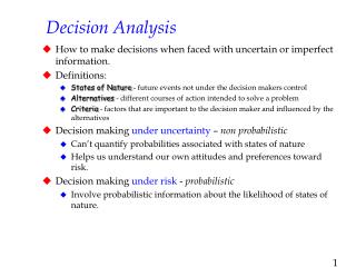
What is Decision Analysis?. Decision analysis is a systematic process of documenting and weighing alternative scenarios in terms of their respective costs, probabilities of success or failure, and benefits. Decision analysis consists of a set of quantitative procedures

What is Decision Analysis?
E N D
Presentation Transcript
What is Decision Analysis? Decision analysis is a systematic process of documenting and weighing alternative scenarios in terms of their respective costs, probabilities of success or failure, and benefits. Decision analysis consists of a set of quantitative procedures that help decision-makers: • structure decision problems and develop creative decision alternatives • combine uncertainty and preferences (values) into a single model to • arrive at optimal decisions • quantify the uncertainty in the processes or outcomes • associated with the decision (this includes combining • existing data and models with expert judgments and beliefs) • quantify their preferences or values (this includes the values of all • stakeholders)
The decision analysis process Identify the decision situation and objectives Identify the alternatives • Decompose and model the problem: • Model of problem structure • Model of uncertainty. • Model of preferences Choose the best alternative Perform sensitivity analysis Is further analysis needed? YES NO Implement the best alternative
Elements of a Decision Problem ·Values are defined simply as the things that matter most to the decision-maker(s). ·An objective is the specific thing that the decision maker wants to achieve. ·The sum of a decision maker’s objectives defines what is important and hence, constitutes his or her values. ·The decision context (or decision situation) is the setting in which the decision occurs. It determines what objectives should be considered. When a series of interrelated sequential decisions must be made, often referred to as dynamic decision situations. ·A requisite decision (Phillips 1982) considers the only the elements that are necessary to solve the problem (i.e., that are relevant within the decision context). Decision alternatives are the options that are available to the decision-maker. ·Uncertain events are the outcomes that could happen in the future due to chance and as a result of a decision. (Only the outcomes that are meaningful to the decision-maker and that have an impact in terms of the objectives should be considered.) ·Consequences are eventual outcomes of the decision situation. Consequences are directly related to the decision-makers objectives (multiple objectives = multiple consequences). The planning horizon is the interval from the current time and current decision to the end of the time line. It should be consistent with the decision context and objectives.
Structuring Decisions ·Once the values, objectives, and decision situation have been identified they need to be put into a logical framework. ·Identify and organize fundamental and means objectives. ·Fundamental objectives are what the decision-maker really wants to accomplish. These are the basis by which the consequences will be measured. ·Means objectives are the things that need to be accomplished to realize the fundamental objective. These are distinguished from the fundamental objectives via the WITI test – Why Is That Important? ·After identifying and structuring the fundamental objectives, we can now structure the remaining elements – decisions and alternatives, uncertain events and outcomes, and consequences.
Means objectives network Have more money How could I achieve this? Fundamental objectives Make more money Spend less money Invest in stocks Buy cheaper brands Get second job Means objectives Why is that important?
Decision alternatives 12”, 14”, 16” minimum length limit Fundamental objectives Satisfy recreational anglers Satisfy tournament anglers Example: Typical Management Decision West Point Reservoir Atlanta The problem Wastewater treatment has decreased fertility Largemouth bass populations have declined Angler catch rates have decreased Anglers and marina operators are dissatisfied 24 22 20 18 16 Adult Largemouth bass CPUE 14 12 10 8 6 1988 1990 1992 1994 1996 1998 Year
What makes LMB anglers happy? Results of 1997 Georgia DNR Statewide Angler Study Recreational LMB angler preferences Limit 1 35 Limit 3 80 Limit 6 60 25 Percent of respondents 40 15 Limit 10 20 5 0 0 12 14 16 18 1 to 5 6 to 10 11 to 15 16 to 20 21 or more Total length (in) Creel limits However, tournament anglers prefer large numbers of legal fish
Structuring Values and Objectives Largemouth bass angler satisfaction Maximize recreational angler satisfaction Maximize tournament angler satisfaction Provide consistent angling opportunities Maximize number of creelable largemouth bass Maximize number of large fish (number of creelable LMB) (number of large LMB) (stable population) (quantifiable objectives = outcomes)
Developing a Model of the Outcomes Recall an earlier model of fishing….. Bait on Hook Fish Hungry Fish caught where the probability of catching a fish is influenced by bait staying on the hook and fish being hungry
Yes No Yes No Yes No Yes No Probability of NOT catching a fish on any given cast Decision Tree Catch Fish 0.80 Fish Hungry Yes 0.50 Yes 0.20 No Bait on Hook 0.50 0.50 Yes No Yes 0.50 0.50 No 0.30 Yes 0.50 No Yes 0.70 No 0.50 0.10 Yes No 0.50 0.90 No Probability of catching a fish on any given cast 0.5*0.5*0.8 + 0.5*0.5*0.5 + 0.5*0.5*0.3 + 0.5*0.5*0.1 = 0.425 + 0.5*0.5*0.9 = 0.575 0.5*0.5*0.2 + 0.5*0.5*0.5 + 0.5*0.5*0.7
Add a Decision to the Tree Catch Fish 0.80 Fish Hungry Yes 0.50 Yes 0.20 No Bait on Hook 0.50 0.50 Yes Probability of catching fish = 0.425 No Yes 0.50 0.50 No 0.30 Yes Cast? 0.50 No Yes Yes 0.70 No 0.50 0.10 Yes No No 0.50 0.90 No Probability of catching fish = 0 Catch Fish 0.00 Yes 1.00 No
Enjoyment Value 1.00*25 = 25.00 … = 56.87 0.00*100 + 0.5*0.5*0.8*100 + 0.5*0.5*0.2*25 Add Values to the Tree Catch Fish 100 0.80 Yes Fish Hungry 0.50 0.20 25 Yes No 0.50 Bait on Hook 100 0.50 Yes No Yes 0.50 25 0.50 No 100 0.30 Yes Cast? 0.50 No Yes 0.70 25 Yes No 0.50 100 0.10 Yes No No 0.50 0.90 25 No Enjoyment Value Catch Fish 0.00 100 Yes 1.00 25 No Enjoyment value of NOT casting Enjoyment value of casting
Add Values to the Net The result: an Influence Diagram
Influence Diagram, 3 basic components The Decision Cast? Bait on Hook Fish Hungry Key Uncertainties (Bayes Network) Catch Fish Enjoyment value Utility
ONLY type of link to represent timing (flow of information) Influence Diagram NOT a flowchart Cast? Bait on Hook Fish Hungry Catch Fish Links represent dependence (causality) Enjoyment value
LMB decision model means objectives network Largemouth bass angler satisfaction How could I achieve this? Fundamental objectives Maximize tournament angler satisfaction Maximize recreational angler satisfaction Maximize number of creelable largemouth bass Provide consistent angling opportunities Means objectives Why is that important? Maximize number of large fish Where do the utility values come from??? For simple (single) endpoints, it’s a simple function of estimated output e.g., animal abundance, number animals harvested. When there are multiple endpoints, need a means to valuate each e.g., the means and objectives hierarchies
Sensitivity analysis Like all models, Bayesian Belief Networks and Influence Diagrams should be examined via sensitivity analysis Basic idea: Vary the values of each parameter and examine the effect on desired outputs Two types of sensitivity analysis Analysis of the influence of parameters on the utility values (IDs only) “value sensitivity comparison” Analysis of the influence of parameters on the probability of a specific outcome (IDs and BBNs) There is no single best method of examining model sensitivity
33.172 Future Fish population Egg-to-Fry-Survival Sediment Yield Current Population Size Watershed Slope 20 22 24 26 28 30 32 34 36 38 40 Net Utility Value Sensitivity Analysis Tornado diagram of timber harvest example Greatest influence Least influence
Aquatic Habitat Model for Interior Columbia River Basin Model
“Probability” Sensitivity Analysis Several measures, most common is known as “entropy reduction” or mutual information Interior Columbia River Basin aquatic habitat model The summary output of the sensitivity analysis of habitat condition node is below Sensitivity of 'Habitat_Condition' due to a finding at another node: Node Mutual Quadratic ---- Info Score Habitat_Condition 1.58310 0.4435845 Ripo_Cond 0.16662 0.0287079 Sed 0.07749 0.0128482 S_G 0.04272 0.0067063 Flood 0.01492 0.0026125 Prior_Ripo_Cond 0.01105 0.0017047 Road_Disturb 0.00474 0.0007314 Future_Grazing 0.00143 0.0002230 Road_Dens 0.00115 0.0001767 Slope_Steepness 0.00041 0.0000635 Fire 0.00000 0.0000000 Grnd_Dist_Index 0.00000 0.0000000 Most Least
These can also be placed in a tornado diagram: Riparian Condition Sediment Standards & Guides Flood Prior Riparian Condition Road Disturbance Future Grazing Road Density Ground Disturbance Index Slope Steepness Fire-Rain 0.00 0.20 0.30 0.50 0.60 0.70 0.10 0.40 Slope 2 Probability of High Aquatic Habitat Capacity “Probability” Sensitivity Analysis The influence of individual nodes on habitat condition probabilities can also be examined Sensitivity of 'Habitat_Condition' to findings at 'Ripo_Cond': Probability ranges: Min Current Max | RMS Change Complex 0.07938 0.3135 0.5415 | 0.1879 Moderately_Simplifie 0.2761 0.3316 0.3917 | 0.04826 Highly_Simplified 0.1508 0.3549 0.6446 | 0.1909 Quadratic scoring = 0.02871 Entropy reduction = 0.1666 (10.5 %)
Management action 9.50 None Low intensity 9.65 High intensity 9.15 Sensitivity analysis suggests that some variables have a greater influence on the net value (utility) of a decision. Consider the following hypothetical of a natural resource management decision analysis. Expected value of management action, Best course of action but not by much bull trout presence unknown, assumed 50/50 Net value is gain from resource use (low/ high) plus value or cost associated future bull trout population status in a sampling frame.
Management action 18.25 None Low intensity 17.25 High intensity 13.75 Value of information Same decision, but presence known Best course of action
Management action 0.75 None Low intensity 2.05 High intensity 5.45 Value of information Same decision, but absence known Best course of action
Management action 0.75 None Low intensity 2.05 High intensity 5.45 Value of Information Draw an arc between the decision and bull trout population: This represents the flow of information. In this instance, knowledge of the presence of bull trout
[0.75] [18.25] None None [2.05] [17.25] Low_intensity Low_intensity [5.45] [13.75] High_intensity High_intensity Expected value of management action when… Bull trout present Bull Trout Absent Optimal value in green
Calculate Value of information The value of PERFECTinformation 18.25*0.500 + 5.45*0.500 = 11.85 11.85 – 9.65 = 2.20
Value of information But… not all information is perfect (it almost never is) Some sources of imperfection Sampling error Incomplete understanding of process Random error Others??? Therefore, we need to consider these when evaluating information
Value of imperfect information, step 1 Let’s say that we want to harvest a watershed that could contain bull trout. We don’t know if it does contain trout and want to know if it’s worth sampling Assume 100 samples are needed to detect bull trout 80% of the time. The Cost of sampling = 0.5 Assume 80% probability of detection: P(detected| present) = 0.80 P(detected| not present) = 0 Assume 50% probability of bull trout present: P(present) = 0.50 P(not present) = 0.50 First we estimate the probability of detecting bull trout if we sampled The probability of detecting bull trout =0.8*0.5 + 0*0.5 = 0.40
P(not detected| present)*P(present) P(not detected| present)*P(present) + P(not detected| not present)*P(not present) 0.20*0.50 = 0.167 or 16.7% 0.20*0.50 + 1*0.50 However, we want to know the (posterior) probability that bull trout are present if not detected (Bayes formula) Assume 80% probability of detection: P(not detected| present) = 1- 0.80 = 0.20 P(not detected| not present) = 1 Assume 50% probability of bull trout present: P(present) = 0.50 P(not present) = 0.50 The posterior probability that bull trout are present Now calculate:
Value of imperfect information, step 2 Notice arrow is reversed representing posterior prob.
Information value is calculated similar to perfect information Value Management activity Sampling decision [9.15] high_intensity Assuming a 50% probability of presence Not sample [9.65] low_intensity [9.65] [9.50] none [10.57] Posterior probability given 50/50 prior and 80% detection probability high_intensity [5.45] Bull trout absent [5.45] low_intensity [2.05] 0.600 none [0.75] Sample [10.57] high_intensity [13.75] Value of sampling information Bull trout present [18.25] [17.25] 10.57 – 9.65 = 0.92 low_intensity 0.400 0.92 minus the cost of collecting samples to get 80% detection probability (0.5) none [18.25] Net = 0.92 – 0.5= 0.42