Download
1 / 16
260 likes | 865 Vues
Solution of a Partial Differential Equations using the Method of Lines. Partial differential equations where there are several independent variables have a typical general form. A problem involving PDE’s requires specification of initial values and boundary conditions.

E N D
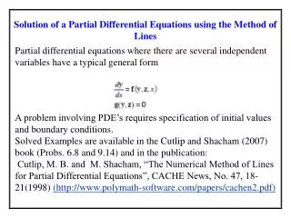
Solution of a Partial Differential Equations using the Method of Lines Partial differential equations where there are several independent variables have a typical general form A problem involving PDE’s requires specification of initial values and boundary conditions. Solved Examples are available in the Cutlip and Shacham (2007) book (Probs. 6.8 and 9.14) and in the publication: Cutlip, M. B. and M. Shacham, “The Numerical Method of Lines for Partial Differential Equations”, CACHE News, No. 47, 18-21(1998) (http://www.polymath-software.com/papers/cachen2.pdf)
Unsteady-state Diffusion and Reaction in a Semi-Infinite Slab Solution by the Method of Lines
Solving Differential-Algebraic System of Equations (DAE’s) using the Controlled Integration Method The system defined by the equations: with the initial conditions y(x0) = y0 is called a system of differential-algebraic equations. Solved examples are available in the Cutlip and Shacham (2007) book (Prob 6.7) and in the reference: Shacham, M., N. Brauner and M. B. Cutlip, "Prediction and Prevention of Chemical Reaction Hazards – Learning by Simulation", Chem. Eng. Educ., 35(4), 268-273(2001) (http://www.polymath-software.com/papers/CEE_35_268_01.pdf)
Stiff Systems of First-Order ODE’s Systems of ODE’s where the dependent variables change on various time (independent variable) scales which differ by many orders of magnitude are called “Stiff” systems. The characterization of stiff systems and the special techniques that are used for solving such systems are described in detail in problem 6.2 in the Cutlip and Shacham (2007) book. Detailed analysis of a problem for stiffness is demonstrated in the publication: Shacham, M., N. Brauner, W. R. Ashurst and M. B. Cutlip, "Can I Trust this Software Package? – An Exercise in Validation of Computational Results ", Chem. Eng. Educ., (in press, 2008) (ftp://ftp.bgu.ac.il/shacham/publ_papers/CEE_08.pdf)
Using MATLAB Symbolic Manipulation Capabilities for Investigation Stiffness of an ODE system Derive the elements of the Jacobian matrix Introduce numerical values into the Jacobian The ratio between the max. and min. eigenvalues of the Jacobian matrix serves as an indicator for the stiffness of the problem
Parameter Estimation in Dynamic Systems The (system) of ordinary differential equations is used to model the data by finding the values of the parameters a0, a1 … an that minimize the squares of the errors Solution of such problems requires the integration of the differential equations in an inner loop in order to obtain the values and minimizing S as function of a0, a1 … an in an outer loop. A solved example is available in the Cutlip and Shacham (2007) book (Prob. 6.9)
ESTIMATING MODEL PARAMETERS INVOLVING ODE’S USING FERMENTATION DATA
ESTIMATING MODEL PARAMETERS INVOLVING ODE’S USING FERMENTATION DATA Data Parameter values Plot of experimental vs. calculated
Nonlinear Programming (Optimization) with Equity Constraints The nonlinear programming problem with equity constrains is defined by: where f is a function, x is an n - vector of variables and h is an m-vector (m<n) of Solution of such problems requires the inclusion of the constraints in the objective function using Lagrange multipliers, differentiating the objective function and solving the resultant system of NLEs. Solved examples are available in the Cutlip and Shacham (2007) book (Probs. 4.5 and 5.5)
Substrate feed rate FI Final volume VI Substrate feed rate FP Final Volume VH Discharge flow rate FH Final Volume VI n – cycle number n = 1 fed-batch operation S (substrate reactant) + X (cell) = P (product) + nX The biochemical reaction is inhibited by the substrate Optimal substrate feed concentration is required with fixed set of operating conditions Three Modes in the Operation of the Semi-batch Bioreactor
Mathematical Physical Properties Model Solution Algorithm Combine Together Models and Algorithms by Programming for Repetitive Runs and Optimization Documentation Solution of Multiple Model – Multiple Algorithm Problems
Three Modes in the Operation of the Semi-batch Bioreactor Results of Ten Cycles of Processing and Harvesting Complete details of the solution can be found in the Cutlip and Shacham (2007) book ( Prob.14.13) and the site: http://www.engr.uconn.edu/~cutlipm/escape17
Skills Needed for Solving Various Types of Problems Introductory Level – Linear Eqs., NLEs, ODE – IVP, Regression 1. Categorize the problem according to the numerical solution technique to be used for its solution. 2. Use one software package (say, POLYMATH) to solve single model – single algorithm problems for one or a few sets of parameter values 3. Use 95% confidence intervals and residual plots to analyze regression results 4. Use a spreadsheet or programming for parametric runs and for preparing graphical and tabular summaries of the results
Skills Needed for Solving Various Types of Problems Advanced Level – NLEs, ODE – BVP, DAE, PDE and Multiple Model – Multiple Algorithm Problems 1. Acquire familiarity with the basic numerical methods for solving NLEs, ODEs, DAEs and PDEs 2. Use programming to combine several algorithms to solve single model multiple algorithm problems (i.e. ODE BVP) 3. Use programming to combine several models to solve multiple model single algorithm problems (i.e. various stages of operation of a reactor) 4. Use programming to combine several models and algorithms to solve multiple model- multiple algorithm problems