Non-Linear Least Squares and Sparse Matrix Techniques: Fundamentals
570 likes | 952 Vues
Non-Linear Least Squares and Sparse Matrix Techniques: Fundamentals. Richard Szeliski Microsoft Research UW-MSR Course on Vision Algorithms CSE/EE 577, 590CV, Spring 2004. Readings. Press et al. , Numerical Recipes, Chapter 15 (Modeling of Data)

Non-Linear Least Squares and Sparse Matrix Techniques: Fundamentals
E N D
Presentation Transcript
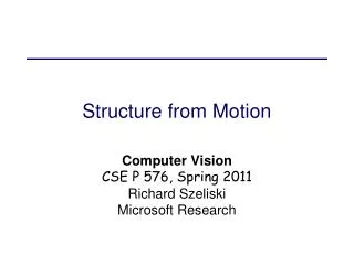
Non-Linear Least Squares and Sparse Matrix Techniques:Fundamentals Richard SzeliskiMicrosoft Research UW-MSR Course on Vision Algorithms CSE/EE 577, 590CV, Spring 2004
Readings • Press et al., Numerical Recipes, Chapter 15 (Modeling of Data) • Nocedal and Wright, Numerical Optimization, Chapter 10 (Nonlinear Least-Squares Problems, pp. 250-273) • Shewchuk, J. R. An Introduction to the Conjugate Gradient Method Without the Agonizing Pain. • Bathe and Wilson, Numerical Methods in Finite Element Analysis, pp.695-717 (sec. 8.1-8.2) and pp.979-987 (sec. 12.2) • Golub and VanLoan, Matrix Computations. Chapters 4, 5, 10. • Nocedal and Wright, Numerical Optimization. Chapters 4 and 5. • Triggs et al., Bundle Adjustment – A modern synthesis. Workshop on Vision Algorithms, 1999. NLS and Sparse Matrix Techniques
Outline • Nonlinear Least Squares • simple application (motivation) • linear (approx.) solution and least squares • normal equations and pseudo-inverse • LDLT, QR, and SVD decompositions • correct linearization and Jacobians • iterative solution, Levenberg-Marquardt • robust measurements NLS and Sparse Matrix Techniques
Outline • Sparse matrix techniques • simple application (structure from motion) • sparse matrix storage (skyline) • direct solution: LDLT with minimal fill-in • larger application (surface/image fitting) • iterative solution: gradient descent • conjugate gradient • preconditioning NLS and Sparse Matrix Techniques
Triangulation – a simple example • Problem: Given some image points {(uj,vj)}in correspondence across two or more images (taken from calibrated cameras cj), compute the 3D location X X (uj,vj) cj NLS and Sparse Matrix Techniques
(Xc,Yc,Zc) uc f u Image formation equations NLS and Sparse Matrix Techniques
Simplified model • Let R=I (known rotation), f=1, Y = vj = 0 (flatland) • How do we solve this set of equations (constraints) to find the best (X,Z)? X uj (xj,zj) NLS and Sparse Matrix Techniques
“Linearized” model • Bring the denominator over to the LHS • or • (Measures horizontal distance to each line equation.) • How do we solve this set of equations (constraints)? X uj (xj,zj) NLS and Sparse Matrix Techniques
Linear regression • Overconstrained set of linear equations • or • Jx = r • where • Jj0=1, Jj1 = -uj • is the Jacobian and • rj = xj-ujzj • is the residual X uj (xj,zj) NLS and Sparse Matrix Techniques
Normal Equations • How do we solve Jx = r? • Least squares: arg minx║Jx-r║2 • E =║Jx-r║2 = (Jx-r)T(Jx-r) • = xTJTJx – 2xTJTr – rTr • ∂E/∂x = 2(JTJ)x – 2JTr = 0 • (JTJ)x = JTr normal equations • A x = b ” (A is Hessian) • x = [(JTJ)-1JT]r pseudoinverse NLS and Sparse Matrix Techniques
LDLT factorization • Factor A = LDLT, where L is lower triangular with 1s on diagonal, D is diagonal • How? • L is formed from columns of Gaussian elimination • Perform (similar) forward and backward elimination/substitution • LDLTx = b, DLTx = L-1b, LTx = D-1L-1b, • x = L-TD-1L-1b NLS and Sparse Matrix Techniques
LDLT factorization – details NLS and Sparse Matrix Techniques
LDLT factorization – details NLS and Sparse Matrix Techniques
LDLT factorization – details NLS and Sparse Matrix Techniques
LDLT factorization – details NLS and Sparse Matrix Techniques
LDLT factorization – details NLS and Sparse Matrix Techniques
LDLT factorization – details NLS and Sparse Matrix Techniques
LDLT factorization – details NLS and Sparse Matrix Techniques
LDLT factorization – details NLS and Sparse Matrix Techniques
LDLT factorization – details NLS and Sparse Matrix Techniques
LDLT factorization – details NLS and Sparse Matrix Techniques
LDLT factorization – details NLS and Sparse Matrix Techniques
LDLT and Cholesky • Variant: Cholesky: A = GGT, where G = LD1/2(involves scalar √) • Advantages: more stable than Gaussian elimination • Disadvantage: less stable than QR: (cond. #)2 • Complexity: (m+n/3)n2 flops NLS and Sparse Matrix Techniques
QR decomposition • Alternative solution for Jx = r • Find an orthogonal matrix Q s.t. • J = Q R, where R is upper triangular • Q R x = r • R x = QTr solve for x using back subst. • Q is usu. computed using Householder matrices, Q = Q1…Qm, Qj = I – βvjvjT • Advantages: sensitivity / condition number • Complexity: 2n2(m-n/3) flops NLS and Sparse Matrix Techniques
SVD • Most stable way to solve system Jx = r. • J = UTΣ V, where U and V are orthogonalΣ is diagonal (singular values) • Advantage: most stable (very ill conditioned problems) • Disadvantage: slowest (iterative solution) NLS and Sparse Matrix Techniques
“Linearized” model – revisited • Does the “linearized” model • which measures horizontal distance to each line give the optimal estimate? • No! X uj (xj,zj) NLS and Sparse Matrix Techniques
Properly weighted model • We want to minimize errors in the measured quantities • Closer cameras (smaller denominators) have moreweight / influence. • Weight each “linearized” equation by current denominator? X uj (xj,zj) NLS and Sparse Matrix Techniques
Optimal estimation • Feature measurement equations • Likelihood of (X,Z) given {ui,xj,zj} NLS and Sparse Matrix Techniques
Non-linear least squares • Log likelihood of (x,z) given {ui,xj,zj} • How do we minimize E? • Non-linear regression (least squares), because ûiare non-linear functions of {ui,xj,zj} NLS and Sparse Matrix Techniques
Levenberg-Marquardt • Iterative non-linear least squares • Linearize measurement equations • Substitute into log-likelihood equation: quadratic cost function in (Δx,Δz) NLS and Sparse Matrix Techniques
Levenberg-Marquardt • Linear regression (sub-)problem: • with • ûi • Similar to weighted regression, but not quite. NLS and Sparse Matrix Techniques
Levenberg-Marquardt • What if it doesn’t converge? • Multiply diagonal by (1 + λ), increase λuntil it does • Halve the step size (my favorite) • Use line search • Other trust region methods[Nocedal & Wright] NLS and Sparse Matrix Techniques
Levenberg-Marquardt • Other issues: • Uncertainty analysis: covariance Σ = A-1 • Is maximum likelihood the best idea? • How to start in vicinity of global minimum? • What about outliers? NLS and Sparse Matrix Techniques
Robust regression • Data often have outliers (bad measurements) • Use robust penalty appliedto each set of jointmeasurements[Black & Rangarajan, IJCV’96] • For extremely bad data, use random sampling [RANSAC, Fischler & Bolles, CACM’81] NLS and Sparse Matrix Techniques
Sparse Matrix Techniques Direct methods
Structure from motion • Given many points in correspondence across several images, {(uij,vij)}, simultaneously compute the 3D location Xi and camera (or motion) parameters (K, Rj, tj) • Two main variants: calibrated, and uncalibrated (sometimes associated with Euclidean and projective reconstructions) NLS and Sparse Matrix Techniques
Bundle Adjustment • Simultaneous adjustment of bundles of rays (photogrammetry) • What makes this non-linear minimization hard? • many more parameters: potentially slow • poorer conditioning (high correlation) • potentially lots of outliers • gauge (coordinate) freedom NLS and Sparse Matrix Techniques
Simplified model • Again, R=I (known rotation), f=1, Z = vj = 0 (flatland) • This time, we have to solve for all of the parameters {(Xi,Zi), (xj,zj)}. Xi uij (xj,zj) NLS and Sparse Matrix Techniques
Lots of parameters: sparsity • Only a few entries in Jacobian are non-zero NLS and Sparse Matrix Techniques
Sparse LDLT / Cholesky • First used in finite element analysis [Bathe…] • Applied to SfM by [Szeliski & Kang 1994] structure | motion fill-in NLS and Sparse Matrix Techniques
Skyline storage [Bathe & Wilson] NLS and Sparse Matrix Techniques
Sparse matrices–common shapes • Banded (tridiagonal), arrowhead, multi-banded • : fill-in • Computational complexity: O(n b2) • Application to computer vision: • snakes (tri-diagonal) • surface interpolation (multi-banded) • deformable models (sparse) NLS and Sparse Matrix Techniques
Sparse matrices – variable reordering • Triggs et al. – Bundle Adjustment NLS and Sparse Matrix Techniques
Sparse Matrix Techniques Iterative methods
Two-dimensional problems • Surface interpolation and Poisson blending NLS and Sparse Matrix Techniques
Poisson blending NLS and Sparse Matrix Techniques
Poisson blending • → multi-banded (sparse) system NLS and Sparse Matrix Techniques
One-dimensional example • Simplified 1-D height/slope interpolation • tri-diagonal system (generalized snakes) NLS and Sparse Matrix Techniques
Direct solution of 2D problems • Multi-banded Hessian • : fill-in • Computational complexity: n x m image • O(nm m2) • … too slow! NLS and Sparse Matrix Techniques