Sparse Matrix Methods
Sparse Matrix Methods. Day 1: Overview Matlab and examples Data structures Ax=b Sparse matrices and graphs Fill-reducing matrix permutations Matching and block triangular form Day 2: Direct methods Day 3: Iterative methods. D. (Demo in Matlab). Matlab sprand spy sparse, full

Sparse Matrix Methods
E N D
Presentation Transcript
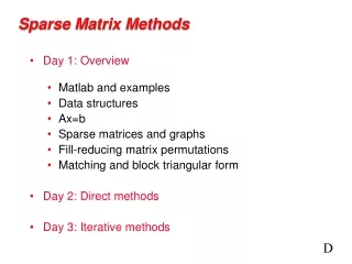
Sparse Matrix Methods • Day 1: Overview • Matlab and examples • Data structures • Ax=b • Sparse matrices and graphs • Fill-reducing matrix permutations • Matching and block triangular form • Day 2:Direct methods • Day 3: Iterative methods D
(Demo in Matlab) • Matlab sprand • spy • sparse, full • matrix arithmetic and indexing • examples of sparse matrices from different applications (from UF site)
Matlab sparse matrices: Design principles • All operations should give the same results for sparse and full matrices (almost all) • Sparse matrices are never created automatically, but once created they propagate • Performance is important -- but usability, simplicity, completeness, and robustness are more important • Storage for a sparse matrix should be O(nonzeros) • Time for a sparse operation should be O(flops)(as nearly as possible)
Data structures • Full: • 2-dimensional array of real or complex numbers • (nrows*ncols) memory • Sparse: • compressed column storage • about (1.5*nzs + .5*ncols) memory D
(Demos in Matlab) • A \ b • Cholesky factorization and orderings
Solving linear equations x = A \ b; • Is A square? no => use QR to solve least squares problem • Is A triangular or permuted triangular? yes => sparse triangular solve • Is A symmetric with positive diagonal elements? yes => attempt Cholesky after symmetric minimum degree • Otherwise => use LU on A(:, colamd(A))
Matrix factorizations in Matlab • Cholesky: • R = chol(A); • simple left-looking column algorithm • Nonsymmetric LU: • [L,U,P] = lu(A); • left-looking “GPMOD”, depth-first search, symmetric pruning • Orthogonal: • [Q,R] = qr(A); • George-Heath algorithm: row-wise Givens rotations
3 7 1 3 7 1 6 8 6 8 4 10 4 10 9 2 9 2 5 5 Graphs and Sparse Matrices: Cholesky factorization Fill:new nonzeros in factor Symmetric Gaussian elimination: for j = 1 to n add edges between j’s higher-numbered neighbors G+(A)[chordal] G(A)
3 7 1 6 8 10 4 10 9 5 4 8 9 2 2 5 7 3 6 1 Elimination Tree G+(A) T(A) Cholesky factor • T(A) : parent(j) = min { i > j : (i,j) inG+(A) } • T describes dependencies among columns of factor • Can compute T from G(A) in almost linear time • Can compute G+(A) easily from T D
(Demos in Matlab) • matrix and graph • elimination tree • orderings in detail
Fill-reducing matrix permutations • Minimum degree: • Eliminate row/col with fewest nzs, add fill, repeat • Theory: can be suboptimal even on 2D model problem • Practice: often wins for medium-sized problems • Nested dissection: • Find a separator, number it last, proceed recursively • Theory: approx optimal separators => approx optimal fill and flop count • Practice: often wins for very large problems • Banded orderings (Reverse Cuthill-McKee, Sloan, . . .): • Try to keep all nonzeros close to the diagonal • Theory, practice: often wins for “long, thin” problems • Best modern general-purpose orderings are ND/MD hybrids.
Fill-reducing permutations in Matlab • Nonsymmetric approximate minimum degree: • p = colamd(A); • column permutation: lu(A(:,p)) often sparser than lu(A) • also for QR factorization • Symmetric approximate minimum degree: • p = symamd(A); • symmetric permutation: chol(A(p,p)) often sparser than chol(A) • Reverse Cuthill-McKee • p = symrcm(A); • A(p,p) often has smaller bandwidth than A • similar to Sparspak RCM D
(Demos in Matlab) • nonsymmetric LU • dmperm, dmspy, components
Matching and block triangular form • Dulmage-Mendelsohn decomposition: • Bipartite matching followed by strongly connected components • Square, full rank A: • [p, q, r] = dmperm(A); • A(p,q) has nonzero diagonal and is in block upper triangular form • also, strongly connected components of a directed graph • also, connected components of an undirected graph • Arbitrary A: • [p, q, r, s] = dmperm(A); • maximum-size matching in a bipartite graph • minimum-size vertex cover in a bipartite graph • decomposition into strong Hall blocks
Complexity of direct methods n1/2 n1/3
Direct A = LU Iterative y’ = Ay More General Non- symmetric Symmetric positive definite More Robust More Robust Less Storage The Landscape of Sparse Ax=b Solvers D
(Demos in Matlab) • conjugate gradients

