Sparse matrix formats
Sparse matrix formats. Outline. In this topic, we will cover: Sparse matrices A row-column-value representation The old Yale sparse matrix data structure Examples Appropriate use. Dense versus sparse matrices. A dense N × M matrix is one where most elements are non-zero


Sparse matrix formats
E N D
Presentation Transcript
Outline In this topic, we will cover: • Sparse matrices • A row-column-value representation • The old Yale sparse matrix data structure • Examples • Appropriate use
Dense versus sparse matrices A dense N × M matrix is one where most elements are non-zero A dense matrix data structure is one that has a memory location allocated for each possible matrix entry • These require Q(NM) memory A sparse matrix is where 90 % or more of the entries are zero • If m is the number of non-zero entries, • The density is m/MN • The row density is m/N • Operations and storage should depend on m • For sparse matrices, m = o(MN)
Example A dense 1 585 478 square matrix of doubles would occupy 18 TiB The matrix representation of the AMD G3 processor has only7 660 826non-zero entries • The density is 0.000003 • The matrix is used for circuit simulation • Simulations requires solving a system of1,585,478 equations in that many unknowns http://www.cise.ufl.edu/research/sparse/matrices/AMD/G3_circuit.html
Dense square matrix data structure This class stores N × Nmatrices with 8 + 4N + 8N2 = Q(N2) bytes class Matrix { private: int N; double **matrix; public: Matrix( int n ); // ... }; Matrix::Matrix( int n ): N( std::max(1, n) ), matrix( new double *[N] ) { matrix[0] = new double[N*N]; for ( inti = 1; i < N; ++i ) { matrix[i] = matrix[0] + i*N; } } pointer arithmetic
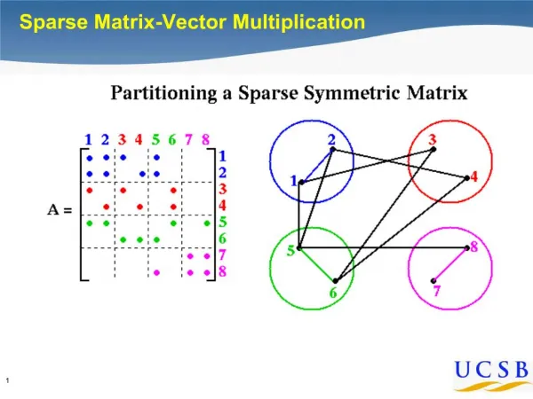
Row-Column-Value Representation As an example: matrix
Row-Column-Value Representation Suppose we store triplets for each non-zero value: • We would have (0, 0, 1.5), (1, 1, 2.3), (1, 3, 1.4), (2, 2, 3.7), … • The class would be class Triplet { int row; int column; double value; };
Row-Column-Value Representation Now the memory requirements are Q(m) class Sparse_matrix { private: intmatrix_size; int N; intarray_capacity; Triplet *entries; public: Sparse_matrix( int n, int c = 128 ); }; Sparse_matrix( int n, intc ): matrix_size( 0 ), N( std::max(1, n) ), array_capacity( std::max(1, c) ), entries( new Triplet[array_capacity] ) { // does nothing }
Row-Column-Value Representation For the same example, we have: entries
Row-Column-Value Representation We fill in the entries in row-major order entries
Row-Column-Value Representation The AMD G3 circuit now requires 117 MiBversus 18 TiB http://www.cise.ufl.edu/research/sparse/matrices/AMD/G3_circuit.html
Accessing Entries Adding and erasing entries (setting to 0) requires a lot of work • They are require O(m) copies entries
Accessing Entries By using row-major order, the indices are lexicographically ordered • We may search using a binary search: O(ln(m)) entries
Old Yale Sparse Matrix Format Storing the row, column, and value of each entry has some undesirable characteristics • Accessing an entry is O(ln(m)) • For the AMD G3, lg(7,660,826) = 23 • If each row has approximately the same number of entries, we can use an interpolation search: O(ln(ln(m))) • For the AMD G3, ln(ln(7,660,826)) = 3
Old Yale Sparse Matrix Format The original (old) Yale sparse matrix format: • Reduces access time to lg(m/N)and uses less memory • For circuits, it is seldom that m/N > 10 • For the AMD G3 circuits, m/N < 5 It was developed by Eisenstatet al. in the late 1970s
Old Yale Sparse Matrix Format Note that the arrays have redundancy • Any row which contains more than one entry is stored in successive entries entries entries 0 1 2 3 4 5 6 7 8 9 10 11
Old Yale Sparse Matrix Format Suppose we store only the location of the first entry of each row: • The first entry in Row 0 is in entry 0 • The first entry in Row 3 is in entry 4 entries 0 1 2 3 4 5 6 7 8 9 10 11
Old Yale Sparse Matrix Format Let us remove that redundancy by creating a new array IA where IA(i) stores the location in JA and A of the first non-zero entry in the ith row • Rename the column and valuearrays to JA and A, respectively IA 0 1 2 3 4 5 6 7 8 0 1 2 3 4 5 6 7 8 9 10 11 JA A
Old Yale Sparse Matrix Format For example, the first entry of the 3rd row is located at position IA(3) IA 0 1 2 3 4 5 6 7 8 0 1 2 3 4 5 6 7 8 9 10 11 JA A
Old Yale Sparse Matrix Format Also, the first entry of the 4th row is located at position IA(4) • The entries of Row 4 are in 4, 5, 6 IA 0 1 2 3 4 5 6 7 8 0 1 2 3 4 5 6 7 8 9 10 11 JA A
Old Yale Sparse Matrix Format Searching for entry ai,jnow only requires you to search double a = 0.0;for ( int k = IA[i]; k < IA[i + 1]; ++k ) { if ( JA[k] == j ) { a = A[k]; } } • For larger row densities, use binary search IA 0 1 2 3 4 5 6 7 8 0 1 2 3 4 5 6 7 8 9 10 11 JA A
Old Yale Sparse Matrix Format Our class could look something like requring28 + 4N + 12m bytes: class Old_yale_sparse_matrix { private: intmatrix_size, N, array_capacity; int *IA, *JA double *A; public: Old_yale_sparse_matrix( int n, int c = 128 ); // other member functions }; Old_yale_sparse_matrix::Old_yale_sparse_matrix( int n, intc ): matrix_size( 0 ), N( std::max(1, n) ), array_capacity( std::max(1,c) ), IA = new int[N + 1]; JA = new int[array_capacity]; A = new double[array_capacity] { for ( inti = 0; i <= N; ++i ) { IA[i] = 0; } }
Old Yale Format: The Zero Matrix We initialize the matrix to the zero matrix IA 0 1 2 3 4 5 6 7 8 0 1 2 3 4 5 6 7 8 9 10 11 JA A
Old Yale Format: Access To demonstrate accessing on the AMD G3 circuit, let us determine the weights of the connections to element 1001 • Looking up the array IA[1001], we note that the results arestored starting at locations 2500, 2501, and 2502 in JA and A IA
Old Yale Format: Access JA A Viewing these two arrays, we have: a1001,1001= 3.09685 a1001,1002= –0.54826 a1001,157003= –2.0
Old Yale Format: Memory Use Storing a sparse 8×8 matrix with 12 non-zero entries: • Full matrix: 8 + 4N + 8N2 = 552 bytes • Row-column-value: 24 + 16m = 216 bytes • Old Yale format: 28 + 4N + 12m = 204 bytes For the AMD G3 circuit where N = 1585478 and m = 7660826 • Full matrix: 8 + 4N + 8N2 = 19 178 324 MiB • Row-column-value: 24 + 16m = 117 MiB • Old Yale format: 28 + 4N + 12m = 94 MiB
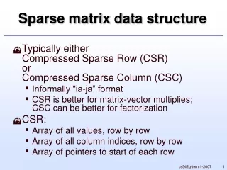
Old Yale Sparse Matrix Format This format is the basis for: • the Harwell-Boeing matrix format, and • the internal representation by Matlab • the new Yale sparse matrix format The first two swap rows and columns... • Old Yale format is row major • Matlab and the Harwell-Boeing are column major
New Yale Sparse Matrix Format The new Yale format makes use of: • diagonal entries are almost always non-zero • the diagonal entries are most-often accessed Thus, store diagonal entries separately:
New Yale Sparse Matrix Format The benefits are quite clear: • Memory usage is less: 28 + 12m bytes • Access to diagonal entries is now Q(1)
New Yale Sparse Matrix Format An implementation of the new Yale sparse matrix format is at http://ece.uwaterloo.ca/~dwharder/aads/Algorithms/Sparse_systems/ This includes: • Constructors, etc. • Matrix and vector functions: norms, trace, etc. • Matrix-matrix and matrix-vector operations • Various solvers: • Jacobi, Gauss-Seidel, forward and backward substitution • Steepest descent, minimal residual, and residual norm steepest descent methods
Operations Suppose that N × Nmatrices have m = Q(N) non-zero entries • At most a fixed number of entries per row Many Q(N2) are reduced to Q(N) run times, including: • Matrix addition—similar to merging • Matrix scalar multiplication • Matrix-vector multiplication • Forward and backward substitution Even finding the M = PLUdecomposition is now O(N2) and not Q(N3)
Operations The M = PLUdecomposition, however, may still be Q(N3) • The worst case is where the firstrow and column are dense • A matrix which has most entriesaround the diagonal is said to bea band diagonal matrix • If all entries are Q(1) of thediagonal, Gaussian elimination andPLU decomposition are Q(N)
Memory Allocation Matlab recognizes this and therefore allows you to specify the initial capacity: >> M = spalloc( N, N, m ); After that, if the array is full, it only assigns room for 10 more entries in the array • This will result in quadratic behaviour if used improperly
Memory Allocation As an experiment, start with an empty 1000 × 1000 sparse matrix and begin assigning entries • After every 10insertions, the array must be resized, and therefore we expect quadratic behaviour • The next plot shows the time required to assign 100 000, 200 000, etc. of those entries
Memory Allocation The least-squares best-fitting quadratic function is a good fit
Memory Allocation Thus, in the previous example, if we pre-allocate one million entries: >> A = spalloc( 1000, 1000, 1000000 );and then fill them, we get linear (blue) behaviour:
Memory Allocation Because the copies are made only every 10 assignments, the effect is not that significant, the number of copies made is only 1/10th of those made if with each assignment:
Sample Test Runs Matlab must maintain the compressed-column shape of the matrix, thus, inserting objects to the left of the right-most non-zero column must consequently require copying all entries over • recall: Matlab’s representation is column-first
Sample Test Runs Thus, this code which assigns m entries: >> n = 1024; >> m = n*n; >> A = spalloc( n, n, m ); >> for j = 1:n % for ( j = 1; j <= n; ++j ) for i = 1:n % for ( i = 1; i <= n; ++i ) A(i, j) = 1 + i + j; end end runs in O(m) time It took 5 s when I tried it
Sample Test Runs While this code, which assigns m entries: >> n = 1024; >> m = n*n; >> A = spalloc( n, n, m ); >> for i = n:-1:1 % for ( i = n; i >= 1; --i ) for j = n:-1:1 % for ( j = n; j >= 1; --j ) A(i, j) = 1 + i + j; end end runs in O(m2) time This took 7 min
Sample Test Runs Even this code which assigns m entries: >> n = 1024; >> m = n*n; >> A = spalloc( n, n, m ); >> for i = 1:n % for ( j = 1; j <= n; ++j ) for j = 1:n % for ( i = 1; i <= n; ++i ) A(i, j) = 1 + i + j; end end also runs in O(m2) time Only half the copies as with theprevious case—just a little less time
Sample Test Runs This is the worst-case order >> n = 1024; >> m = n*n; >> A = spalloc( n, n, m ); >> for j = n:-1:1 for i = n:-1:1 A(i, j) = 1 + i + j; end end I halted the computer after 30 min
Sample Test Runs Consequently, it is your responsibility to use this data structure correctly: • It is designed to allow exceptionally fast accesses, including: • Fast matrix-matrix addition • Fast matrix-vector multiplication • Fast Gaussian elimination and backward substitution
Example Consider the following circuit with resistors and operational amplifies This is from an example in Vlach and Singhal, p.143.
Example The modified nodal representation of the circuit is represented by this sparse matrix: recover the original matrix I0 0 1 2 3 4 5 6 7 0 1 2 3 4 5 6 7 8 9 10 11 12 13 14 15 16 17 18
Example It is a conductance matrix with op amps and is therefore square and not symmetric • The IA matrix has size 7 = N + 1 entries • The matrix is 7 × 7 • The last entry of IA is 19 • There are 19 non-zero entries 0 1 2 3 4 5 6 7 0 1 2 3 4 5 6 7 8 9 10 11 12 13 14 15 16 17 18
Example We will build the matrix row-by-row 0 1 2 3 4 5 6 7 0 1 2 3 4 5 6 7 8 9 10 11 12 13 14 15 16 17 18
Example Row 0 is stored in entries 0 and 1 IA[0]throughIA[1] – 1 with entries 0.1 in column 0 -0.1 in column 1 0 1 2 3 4 5 6 7 0 1 2 3 4 5 6 7 8 9 10 11 12 13 14 15 16 17 18
Example Row 0 is stored in entries 0 and 1 IA[0]throughIA[1] – 1 with entries 0.1 in column 0 –0.1 in column 1 0 1 2 3 4 5 6 7 0 1 2 3 4 5 6 7 8 9 10 11 12 13 14 15 16 17 18
Example Row 1 is stored in entries 2 through 5 IA[1]throughIA[2] – 1 with entries -0.1 in column 0 0.6 in column 1 -0.5 in column 2 1.0in column 6 0 1 2 3 4 5 6 7 0 1 2 3 4 5 6 7 8 9 10 11 12 13 14 15 16 17 18