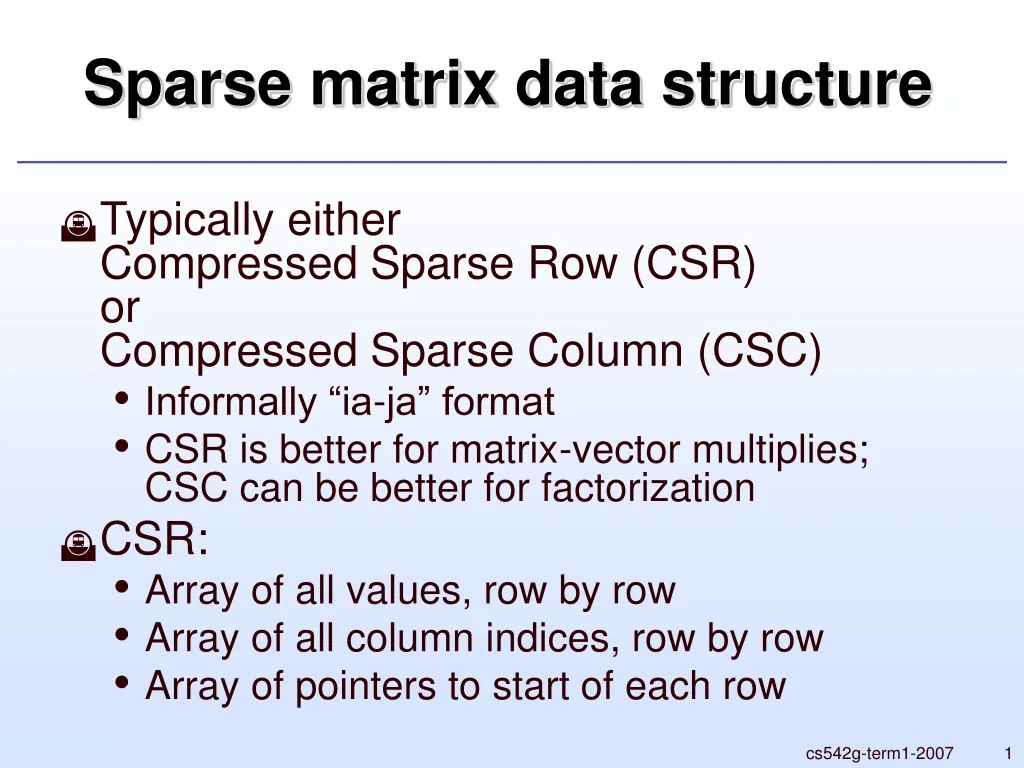
1. Sparse matrix data structure • Typically eitherCompressed Sparse Row (CSR)orCompressed Sparse Column (CSC) • Informally “ia-ja” format • CSR is better for matrix-vector multiplies; CSC can be better for factorization • CSR: • Array of all values, row by row • Array of all column indices, row by row • Array of pointers to start of each row cs542g-term1-2007

2. Direct Solvers • We’ll just peek at Cholesky factorization of SPD matrices: A=LLT • In particular, pivoting not required! • Modern solvers break Cholesky into three phases: • Ordering: determine order of rows/columns • Symbolic factorization: determine sparsity structure of L in advance • Numerical factorization: compute values in L • Allows for much greater optimization… cs542g-term1-2007

3. Graph model of elimination • Take the graph whose adjacency matrix matches A • Choosing node “i” to eliminate next in row-reduction: • Subtract off multiples of row i from rows of neighbours • In graph terms: unioning edge structure of i with all its neighbours • A is symmetric -> connecting up all neighbours of i into a “clique” • New edges are called “fill”(nonzeros in L that are zero in A) • Choosing a different sequence can result in different fill cs542g-term1-2007

4. Extreme fill • The star graph • If you order centre last, zero fill: O(n) time and memory • If you order centre first, O(n2) fill: O(n3) time and O(n2) memory cs542g-term1-2007

5. Fill-reducing orderings • Finding minimum fill ordering is NP-hard • Two main heuristics in use: • Minimum Degree: (greedy incremental)choose node of minimum degree first • Without many additional accelerations, this is too slow, but now very efficient: e.g. AMD • Nested Dissection: (divide-and-conquer)partition graph by a node separator, order separator last, recurse on components • Optimal partition is also NP-hard, but very good/fast heuristic exist: e.g. Metis • Great for parallelism: e.g. ParMetis cs542g-term1-2007

6. A peek at Minimum Degree • See George & Liu, “The evolution of the minimum degree algorithm” • A little dated now, but most of key concepts explained there • Biggest optimization: don’t store structure explicitly • Treat eliminated nodes as “quotient nodes” • Edge in L= path in A via zero or more eliminated nodes cs542g-term1-2007

7. A peek at Nested Dissection • Core operation is graph partitioning • Simplest strategy: breadth-first search • Can locally improve with Kernighan-Lin • Can make this work fast by going multilevel cs542g-term1-2007

8. Theoretical Limits • In 2D (planar or near planar graphs), Nested Dissection is within a constant factor of optimal: • O(n log n) fill (n=number of nodes - think s2) • O(n3/2) time for factorization • Result due to Lipton & Tarjan… • In 3D asymptotics for well-shaped 3D meshes is worse: • O(n5/3) fill (n=number of nodes - think s3) • O(n2) time for factorization • Direct solvers are very competitive in 2D, but don’t scale nearly as well in 3D cs542g-term1-2007

9. Symbolic Factorization • Given ordering, determining L is also just a graph problem • Various optimizations allow determination of row or column counts of L in nearly O(nnz(A)) time • Much faster than actual factorization! • One of the most important observations:good orderings usually results in supernodes: columns of L with identical structure • Can treat these columns as a single block column cs542g-term1-2007

10. Numerical Factorization • Can compute L column by column with left-looking factorization • In particular, compute a supernode (block column) at a time • Can use BLAS level 3 for most of the numerics • Get huge performance boost, near “optimal” cs542g-term1-2007

11. Software • See Tim Davis’s list atwww.cise.ufl.edu/research/sparse/codes/ • Ordering: AMD and Metis becoming standard • Cholesky: PARDISO, CHOLMOD, … • General: PARDISO, UMFPACK, … cs542g-term1-2007