Snow depth reconstruction using UAV-based Lidar and Photogrammetry
30 likes | 197 Vues
Ben Vander Jagt 1 , Michael Durand 1 , Arko Lucieer 2 , Darren Turner 2 , Luke Wallace 2 bvanderj@gmail.com 1 School of Earth Sciences, The Ohio State University 2 School of Geography, University of Tasmania. AGU Annual Conference– Dec, 2013 Moscone Convention Center San Francisco, CA.

Snow depth reconstruction using UAV-based Lidar and Photogrammetry
E N D
Presentation Transcript
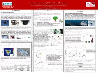
Ben Vander Jagt1, Michael Durand1, Arko Lucieer2, Darren Turner2, Luke Wallace2bvanderj@gmail.com 1 School of Earth Sciences, The Ohio State University 2School of Geography, University of Tasmania AGU Annual Conference– Dec, 2013 Moscone Convention Center San Francisco, CA • 1. Introduction • Unmanned Aerial Vehicles (UAV’s) • Remote sensing technology has improved a great deal in recent decades and the miniaturizationof sensors and positioning systems has paved the way for the use of Unmanned Aerial Vehicles (UAVs) for a wide range of environmental remote sensing applications. . The datasets producedby UAV remote sensing are at such high detail that characteristics of the landscape can be • mapped that are simply not distinguishable at the resolutions generally obtainable via manned aircraft and satellite systems. Furthermore, the ease of deployment and low running costs of theUAVsystems allows for frequent missions providing very high spatial and temporal resolution datasets on-demand. • Figure 1: Common UAV platforms, such as multirotor helicopters (left)can be used to produce high quality remote sensing products using off-the-shelf imaging cameras(middle) and low cost lidar (right). These platforms can be operated remotely via radio link, and/or autonomously using an onboard navigation system. • B. Remote Sensing of Snowpack • Snow is a principle component of the hydrologic budget in many parts of the world, thus being able to make measurements of snow parameters over a spatially continuous area has both civil and scientific merit. The scale of spaceborne measurements often presents unique challenges • due to subpixelvariability of differentvariableswhichcontribute to the measurement (e.g. microwave remote sensing). In situ measurements, while accurate, do notcapture the spatialheterogeneity of the snowpack. • Figure 2: Typical snow depth measurements are discrete in nature (rather than spatially continuous), and often expose field personnel to environments with risk factors including avalanches and extreme weather, • 2. Methods • Collinearity Equations • The collinearity equations relate the measured image coordinates in the 2D camera • coordinate system to those in the “real world” 3D Cartesian coordinate system in the • following manner. • - image coordinates of conjugate points. • - Elements of rotation matrix describing the camera orientation parameters • - Object space coordinates of camera exposure station • - Interior orientation parameters of camera (known from calibration) • - Object space coordinates of target (snow surface) • B. Space Intersection • The method for determining the 3D location of diff- • erent target points from image measurements is • known in conventional analytical photogrammetry as • the space intersection. Assuming the position and • orientation of the camera at the time of exposure is • known for a stereopair (i.e. using a GPS/IMU • solution), the 3D “real world” position of an • identifiable feature can be computed, provided that • image coordinates are measured in a minimum of two • photographs. The standard model used for this • calculation is based on the well-known collinearity • equations, which were briefly described above. The • expression simply relates measured image • coordinates of an object A to the 3D object space • coordinates of A. • Figure 4: A diagram of the photogrammetric space intersection • is shown above. Using a minimum of two images with • covisible points (top right), the 3D coordinates of the snow • surface can be determined (bottom right). • C. Lidar and Lidar Equation • Lidar is a remote sensing technology that measures distance by illuminating a target with a • laser and analyzing the reflected light. Accurate ranging can be accomplished by recording the time-of-flight. The position and orientation of the scan system is need to construct and orient the point cloud. Accurate timing is arguably the most important component of lidar data collection • -3D coordinates of object point in mapping frame • -3D object coordinates in the laser frame • -Rotation matrix from INS to mapping frame • -Rotation matrix from laser to INS frame • -Lever arm offset in INS frame • - 3D coordinates of INS in mapping frame • Figure 5: A diagram of the lidar measurement. If the position, • orientation, and time is known, 3D points of the surface can be determined. The accuracy of the point cloud is dependent on the quality of your GPS/IMU solution. • C. Snow Depth Observations • To validate our methodologies, we measured snow depth at 37 spatially distributed locations • within our study area. Using RTK GPS, we first measured the snow surface at a point, after which the ground surface was measured. The snow depth was calculated by differencing the two observations. The measurement accuracy is ~3cm RMSE. • 3. Results • 3D Point Clouds from Lidar and Photogrammetry • While the output of the lidar equation are points directly mapped into a 3D object space coord- inate system, the point cloud derived from photogrammetric techniques requires additional processing. The camera poses and a sparse point cloud is first produced as output from the bundle adjustment. Once the camera poses are estimated, a dense point cloud can be generated by iteratively matching all covisiblepixels in the images via the epipolar condition, and calculating the object space coordinates via the collinearity equations. • Figure 6: Point clouds of the snow surface at different stages of processing. The lidar derived clouds are immediatedly available at their densest resolution(left), whereas the photogrammetric derived cloud is transformed from sparse to dense after the bundle adjustment is performed. • B. Accuracy Validation with and without ground control • While there exists enough texture in the images of the snow covered ground to determine feature points and run the subsequent bundle adjustment, the point clouds themselves are of no use, unless they are accurately geo-registered to the ground surface. To validate, we measured the coordinates of ground control targets in the image, and compared the true values to those found in both the lidar and photogrammetric point cloud. • Figure 7: Errors in the different observation methodologies when • compared to ground control points measured with GNSS. • Simulated Depth Measurements (Based on accuracy assessment) • Unfortunately, due to calibration issues and travel obligations, there hasn’t been a snow free data collection at the field site. Therefore, we can only simulate what the errors in depth would look like based on our accuracy assessment. Because the vertical errors were biased, any diff- erencing should in fact remove the bias, leaving true snow depth. • Figure 8: Plots of the true vs. esti- mated depths are shown for phot- grammetry (left) and lidar (right). Plots are shown with (blue) and without (green) the bias removed. • 5. Conclusions • This poster has outlined the methodology that one could employ to generate accurate spatially continuous estimates of snow depth from low-cost UAV-acquired imageryand lidar. Point clouds have absolute accuracies in the range of 10–19 cm, depending on the technique used. Relative accuracies are much higher, and we believe the bias is resulting from system calibration error. • Acknowledgment • This study was funded with an NSF East Asia and Pacific Studies Institute (EAPSI) fellowship, award # OISE-1310711. The author wishes to personally thank his colleagues at University of Hobart for their hospitality, time, and effort. This study would not be possible without their support. We also wish to acknowledge Nora May for the use of several figures used in the poster. • References • 1. May, N. A Rigorous approach to comprehensive performance analysis of state of the airborne mobile mapping systems. Ph.Ddissertation. The Ohio State University 2008. • 2. Kraus, K. Photogrammetry: Geometry from Images and Laser Scans, Volume 1. 2nd Edition. Walter de Gruyter, 2007 • 3. Lowe, David G. "Object recognition from local scale-invariant features."Computer vision, 1999. The proceedings of the seventh IEEE international conference on. Vol. 2. Ieee, 1999. • 4. Wallace, L., Lucieer, A., Watson, C., & Turner, D. (2012). Development of a UAV-LiDAR system with application to forest inventory. Remote Sens, 4(6), 1519-1543. Snow depth reconstruction using UAV-based Lidar and Photogrammetry • 2. Study Area and Datasets • Our study site was located in Mount Field National Park, Tasmania, near the summit of Mount Mawson. We chose the site because it is characteristic of typical alpine environments with • steepslopes, high winds, anddeepsnow pack. • Figure 3: Inset of Mount Field Nat’l Park, located in South Central Tasmania (left). Also shown is an ortho- • mosaic of our field site(right). The total size of our study area was approximately 1 hectare. • Datasets • Lidar and digital images were collected over the study area during two flights. The position andorientationof the lidar and camera were observed and time-stamped using a dual-frequency GNSS receiver fused with a IMU. The navigation solution consisted of a loosely-coupled • Sigma Point Kalman Filter. The GNSS observations were differentially post-processed to yield estimated coordinate accuracies in the 2-4 cm range at the antenna. • We used commercially available off-the- • shelf products which are widely available • to demonstrate the practicality of such a • platform for snow depth retrieval. • Table 1: Manufacturer, model, and estimated cost of sensors used in this study.