Download
1 / 11
110 likes | 327 Vues
Understanding the Performance of TCP Pacing. Amit Aggarwal, Stefan Savage, Thomas Anderson Department of Computer Science and Engineering University of Washington. B. TCP Overview:. TCP is a sliding window-based algorithm. Ack-clocking. Slow-start phase (W=2*W each RTT).

E N D
Understanding the Performance of TCP Pacing Amit Aggarwal, Stefan Savage, Thomas Anderson Department of Computer Science and Engineering University of Washington
B TCP Overview: • TCP is a sliding window-based algorithm. • Ack-clocking. • Slow-start phase (W=2*W each RTT). • Congestion-avoidance phase (W++ each RTT). • Slow Start • Losses • Ack compression • Multiplexing TCP Burstiness:
Motivation: • From queuing theory, we know that bursty traffic produces: • Higher queuing delays. • More packet losses. • Lower throughput. Random Worst Case Best Case Response Time 1 Queue Capacity Load
Contribution: • Evaluate the impact of evenly pacing TCP packets across a round-trip time. What to expect from pacing TCP packets? • Better for flows: • Since packets are less likely to be dropped if they are not clumped together. • Better for the network: • Since competing flows will see less queuing delay and burst losses.
Simulation Setup: 4x Mbps 5 ms R1 S1 • Jain’s fairness index f: f = ( xi)2 ( xi RTTi)2 n xi2 n (xi RTTi)2 B= x Mbps 40 ms S pkts 4x Mbps 5 ms Sn Rn
Experimental Results: • A) Single Flow: case S=0.25*B*RTT TCP Reno due to its burstiness in slow-start, incurs a loss when W=0.5*B*RTT paced TCP incurs its first loss after it saturates the pipe, I.e when W=2*B*RTT As a result, TCP Renotakes more time in congestion avoidance to ramp up to B*RTT (paced TCP achieves better throughput only at the beginning) case SB*RTT (They both achieve similar throughput) The bursty behavior of TCP Reno is absorbed by the buffer and it does not get a loss until W=B*RTT
B) Multiple Flows: 50 flows starting at the same time. All flows have same RTT. case S=0.25*B*RTT (TCP Reno achieves better throughput at the beginning!) (Paced TCP achieves better throughput in steady-state!) TCP Reno Flows send bursts of packets in clusters; some drop early and backoff, allowing the others to ramp up. paced TCP All the flows first saturate the pipe. At this point everyone drops because of congestion and mixing of flows, thereby leaving the bottleneck under-utilized. (Synchronization effect) In steady state, all packets are spread out and flows are mixed; as a result there is a randomness in the way packets are dropped. During a certain phase, some flows might get multiple losses, while others might get away without any. (De-synchronization effect) case SB*D De-synchronization effect of Paced TCP persists.
C) Multiple Flows - Variable RTT: 50 flows starting at the same time. 25 flows have RTT=100 msec and 25 flows with RTT=280 msec. case S=0.25*B*RTT (Paced TCP achieves better fairness without sacrificing throughput) TCP Reno the higher burstiness as a result of overlap of packet clusters from different flows becomes visible. It has a higher drop rate at the bottleneck link while achieving similar throughput. case SB*D TCP Reno higher drop rate persists.
D) Variable Length Flows: A constant size flow is established between each of 20 senders and corresponding 20 receivers. As a particular flow finishes, a new flow is established between the same nodes after an exponential think time of mean 1 sec. Ideal-latency: the latency of a flow that does slow start until it reaches its fair share of the bandwidth and then continues with a constant window. (just for comparison reasons) Phase1: no losses. Latency of paced TCP slightly higher due to pacing. Phase 2: S=0.25*B*RTT TCP Reno experience more losses in slow start; some flows timeout. Case SB*Dthis effect disappears. Phase 3: Synchronization effect of paced TCP is visible. Phase 4: Synchronization effect disappears because flows are so large that new flows start infrequently.
E) Interaction of Paced and non-paced flows: A paced flow is very likely to experience loss as a result of one of its packets landing in a burst from a Reno flow. Reno flows are less likely to be affected by bursts from other flows. Result: TCP Reno have much better latency than paced flows, when both are competing for bandwidth in a mixed flow environment. If we continuously instantiate new flows, the performance of paced TCP even deteriorates more. New flows in slow start, cause the old paced flows to regularly drop packets, further diminishing the performance of pacing.
Conclusion:: Pacing improves fairness and drop rates. Pacing offers better performance with limited buffering. In other cases; pacing leads to performance degradation due to: 1. Pacing delays the congestion signals to a point where the network is already over subscribed. 2. Due to mixing of traffic pacing synchronizes drops.