Performance models of TCP

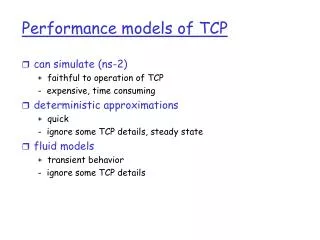
1. Performance models of TCP • can simulate (ns-2) + faithful to operation of TCP - expensive, time consuming • deterministic approximations + quick - ignore some TCP details, steady state • fluid models + transient behavior - ignore some TCP details

2. TCP behavior TCP runs at end-hosts • congestion control: • decrease sending rate when loss detected, increase when no loss • routers • discard, mark packets when congestion occurs • interaction between end systems (TCP) and routers? • want to understand (quantify) this interaction congested router drops packets

3. Generic TCP behavior • window algorithm (window W ) • up to W packets in network • return of ACK allows sender to send another packet • cumulative ACKS • increase window by one per RTT W <- W +1/W perACK  W <- W +1 per RTT • seeks available network bandwidth

4. receiver W sender

5. Generic TCP behavior • window algorithm (window W) • increase window by one per RTT W <- W +1/W per ACK • loss indication of congestion • decrease window by half on detection of loss, (triple duplicate ACKs), W <- W/2

6. receiver TD sender

7. Generic TCP Behavior • window algorithm (window W) • increase window by one per RTT W <- W +1/W per ACK • halve window on detection of loss, W <- W/2 • timeouts due to lack of ACKs -> window reduced to one, W <-1

8. TO receiver sender

9. Generic TCP Behavior • window algorithm (window W) • increase window by one per RTT (or one over window per ACK, W <- W +1/W) • halve window on detection of loss, W <- W/2 • timeouts due to lack of ACKs, W <-1 • successive timeout intervals grow exponentially longup to six times

10. Idealized model: W is maximum supportable window size (then loss occurs) TCP window starts at W/2 grows to W, then halves, then grows to W, then halves… one window worth of packets each RTT to find: throughput as function of loss, RTT TCP throughput/loss relationship loss occurs W TCP window size W/2 time (rtt)

11. TCP throughput/loss relationship # packets sent per “period” = W TCP window size W/2 period time (rtt)

12. TCP throughput/loss relationship # packets sent per “period” = W TCP window size W/2 period time (rtt)

13. 1 packet lost per “period” implies: ploss or: TCP throughput/loss relationship # packets sent per “period” W TCP window size W/2 period time (rtt) B throughput formula can be extended to model timeouts and slow start (PFTK)

14. Recall RED queue management • dropping/marking packets depends on average queue length -> p = p(x) • More generally: active queue management (AQM) 1 Marking probability p pmax 0 tmin tmax 2tmax Average queue length x

15. iBi(RTTi ,p) = C C -router bandwidth Bi - throughput of flow i Bottleneck behavior bottleneck router: • capacity fully utilized • all interfering sessions see same loss prob. • do all sessions see same thruput?

16. Single bottleneck: infinite flows • N infinite TCP sessions • two way propagation delay Ai, i = 1,…,N • throughput Bi(p,RTTi) • one bottleneck router • RED queue management • avg. queue length x ; dropping probability p(x) • to discover • Bi: TCP sessions’ throughput, • router behavior, e.g., drop prob. avg. queue len.

17. i Bi(x) = C, for i =1 ,…,N Model and solution • model • solve a fixed point problem for x • unique solution provided B is monotonic and continuous on x • resulting x can be used to obtain RTTi and p p = p(x) (AQM) RTTi= Ai + x /C (round trip time) i B (p , RTT i) = C, for i =1 ,…,N

18. Model versus simulation: single bottleneck, infinite flows • fixed router capacity 4 Mbps and RED parameters • 10-120 TCP flows • two-way prop. delay 20+2i ms, i = 1,…,N router loss throughput

19. Bnew(p) thruput BTCP(p) p Bottleneck principle: a qualitative result • new/improved, Bnew(p) • TCP, BTCP(p) Bnew(p) > BTCP(p)

20. C Nnew NTCP p Sharing bottleneck with TCP Nnew Bnew(p)+ NTCP Bni(p) = C  Bnew(p) > BTCP(p) • a win! friendly?

21. C N pTCP pnew Replacing TCP with TCP-new NBnew(pnew)= C vs NBTCP(pTCP)= C  pnew >pTCP • a loss!

22. simple model for TCP c ≈ 1.2 • bottleneck principle • multiple bottlenecks • fluid models

23. N TCP flows throughputs B = <Bi (Ri,pi)> V congested AQM routers capacities C = <Cv > avg. queue lengths x = <xv > discard prob. p = <pv (xv )> Multiple Bottleneck: infinite flows bottleneck router model iBi(x) = Cv , v =1,…,V V equations, V unknowns

24. Results: multiple bottleneck, infinite flows • tandemnetwork core, 5 -10routers • 2-way propagation delay20-120ms • bandwidth, 2-6 Mbps • PFTK model error • throughput < 10% • loss rate < 10% • avg. queue length < 15% • similar results for cyclic networks throughput router loss

25. Comments • what about UDP / non-TCP flows? • If there are “non-responsive” flows, just decrease bottleneck capacity by non-responsive flow rate • what about short lived flows? • Hard (some work in sigcomm 2001 – massoulie) • note: throughout, assumption that time to send packets in window is less that RTT

26. Dynamic (transient) analysis of TCP fluids • model TCP traffic as fluid • describe behavior of flows and queues using Ordinary Differential Equations • solve resulting ODEs numerically

27. Packet Drop/Mark Round Trip Delay (t) Loss Model AQM Router B(t) p(t) Sender Receiver Loss Rate as seen by Sender: l(t) = B(t-t)*p(t-t)

28. A Single Congested Router • focus onsingle bottlenecked router • capacity {C (packets/sec)} • queue length q(t) • discard prob. p(t) • N TCP flows thru router • window sizes Wi(t) • round trip time Ri(t) = Ai+q(t)/C • throughputs Bi(t) = Wi(t)/Ri(t) TCP flow i AQM router C, p

29. - q(t) - x(t) t -> Adding RED to the model RED: Marking/dropping based on average queue length x(t) 1 Marking probability p pmax tmin tmax 2tmax Average queue length x x(t): smoothed, time averaged q(t)

30. System of Differential Equations Timeouts and slow start ignored Window Size: Loss arrival rate Mult. decrease Additive increase Queue length: Outgoing traffic Incoming traffic

31. Loss probability: Where dp is obtained from the marking profile dx System of Differential Equations (cont.) Average smoothed queue length: Where a = averaging parameter of RED(wth) d = sampling interval ~ 1/C

32. N+2 coupled equations N flows Wi(t) = Window size of flow i Ri(t) = RTT of flow i p(t) = Drop probability q(t) = queue length Equations solved numerically using MATLAB

33. Steady slate behavior • let t → ∞ • this yields • the throughput is

34. A Queue is not a Network Network - set of AQM routers, V sequence Vi for sessioni Round trip time - aggregate delay Ri(t)=Ai+ SvViqv(t) Loss/marking probability -cumulative prob pi (t)= 1-PvVi(1 - pv(qv(t))) Link bandwidth constraints Queue equations

35. 2600 j 2600 j 1300  j t=30 t=90 How well does it work? • OC-12 – OC-48 links • RED with target delay 5msec • 2600 TCP flows OC-12 OC-48 • decrease to 1300 at 30 sec. • increase to 2600 at 90 sec.

36. simulation fluid model instantaneous delay time (sec) Good queue length match

37. window size average window size simulation fluid model simulation fluid model time (sec) time (sec) matches average window size

38. OC-12 OC-12  j OC-48  j OC-48 2600 j 2600 j 1300 j 2600 2600 1300 t=30 t=90 t=30 t=90 Scaling Properties Wk(t) = Wjk(t) qv(t) = qjv(t)/100

39. What have we seen? model TCP as constant rate fluid flows rate sensitive to congestion via: capacities C = <Cv > avg. queue lengths x = <xv > discard prob. p = <pv (xv )> dynamic (transient) behavior of TCP modeled as system of differential equations Summary: TCP flows as fluids ability to predict performance of system of TCP flows using fluid models