Download
1 / 21
210 likes | 256 Vues
Discussion of probability rules, binomial distribution, relative frequency approach, probability models, and key rules for calculating probabilities. Learn through examples and mathematical notation.

E N D
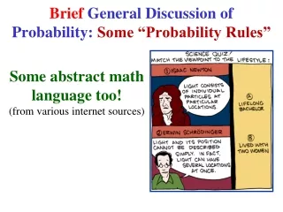
Brief General Discussion of Probability: Some “Probability Rules” Some abstract math language too! (from various internet sources)
Some comments! • There are huge numbers of discrete probability distributions which are NOT BINOMIAL! • So, when given a problem, don’t automatically assume that you should use the binomial distribution! • The binomial distribution only applies when there are just 2 possible outcomes of each event.
Probability The Science of Random Behavior • Random behavior is unpredictable for an individualobject, but it has a regular and predictable patternon the averagefor a huge number of objects. • This is why we can use probability to gain useful results from random samples & randomized comparative experiments.
Probability Theory • Math Description of Randomness • Random Individual outcomes are uncertain but there is a regular distribution of outcomes in a large number of repetitions. • This is why we can use probability to gain useful results from random samples & randomized comparative experiments.
For a random phenomenon, the probability of any outcome Proportion of times the outcome would occur in a very long series of repetitions. • This is called the Relative Frequencyapproach to probability theory. • For many events, the relative frequency of a given outcome settles down to one value over the long run. That one valueis then defined to be the probabilityof that outcome.
Relative Frequency The proportion of occurrences of an outcome. It settles down to one value over the long run. That one valueis then defined to be the probabilityof that outcome. • Relative Frequency Probabilitiescan be determined (checked) by observing a long series of independent trials (empirical data): • Do experiments with many samples • Do simulations, with computers, with random number tables, etc.
Example: Flipping a Fair Coin NOTE! The binomial distribution does applyto this problem!
Probability Models • The sample space Sof a random phenomenon is the set of all possible outcomes. • An event is an outcome or a set of outcomes (a subset of the sample space). • A probability modelis a mathematical description of long-run regularity consisting of a sample space Sand a method of assigning probabilitiesto events.
Probability Model for Two Fair Dice Random Phenomenon Example: Roll a pair of fair dice. The Sample Spaceis illustrated in the figure: The probabilities of each individual of the 36 outcomes are found by inspection. Each clearly occurs with a probability: p = (1/36) = 0.0278
Probability Model for Two Fair Dice • Roll a pair of fair dice. The Sample Spaceis • illustrated in the figure: • The probabilities of each of the 36 possible outcomes is • p = (1/36) = 0.0278 • I’m showing this to drive home the point that • the probability distribution for two dice is • NOT BINOMIAL!
Probability Rule #1: AllProbabilities Must BeNumbers Between 0 & 1. • A probability can be interpreted as the proportion of times that a certain event can be expected to occur. • So, if the probability of an event is more than 1, then it will occur more than 100% of the time!! This is clearly illogical & impossible!
Probability Rule #2: The sum of the probabilities of all possible outcomes must be 1. • Because some outcome must occur on every trial, the sum of the probabilities for all possible outcomes must be exactly one. • If the sum of all of the probabilities is less than one or greater than one, then the resulting probability model will be incoherent & illogical.
Probability Rule #3: • If two events have no outcomes in common,they are said to be disjoint. • The probability that one or the other of two disjoint events occurs is the sum of their individual probabilities.
Example of Disjoint Probabilities: • If two events have no outcomes in common, they are said to be disjoint. Probability that one or the other of 2 disjoint events occurs = sum of individual probabilities. • Consider data about the age distribution of women at first child birth. Obviously, the sample population is women who have had children! • So, it excludes women with no children!
Note: By Rule #3 (or Rule #2) This must be 42% A study of census data for women gives: Under 20:25%. 20-24: 33%.25+:? • So, the probabilitythat a woman in the • sample population who is 24 or youngerhas had a first child is: • = 25% + 33% = 58%
Probability Rule #4: The probability that an event does not occur 1 minus the probability that the event does occur. • Example: As a jury member, you assess the probability that the defendant is guilty to be 0.8. So, you must also believe that the probability the defendant is not guilty is 0.2 in order to be consistent. • Similarly, if the probability that a flight will be on time is 0.7, then the probability it will be late is 0.3.
Consider again the Random Phenomenon of rolling a pair of fair dice. As we’ve already seen, The Sample Spaceis illustrated in the figure: The probabilities of each individual of the 36 outcomes are found by inspection. Each clearly occurs with a probability: p = (1/36) = 0.0278
All possible outcomesof rolling a pair of fair dice are shown in the figure. Calculate the probability P(5) of rolling a 5.
All possible outcomesof rolling a pair of fair dice are shown in the figure. Calculate the probability P(5) of rolling a 5. P(5) P( ) + P( ) + P( ) + P( ) =
All possible outcomesof rolling a pair of fair dice are shown in the figure. Calculate the probability P(5) of rolling a 5. P(5) P( ) + P( ) + P( ) + P( ) = (1/36) + (1/36) + (1/36) + (1/36) = (4/36) = (1/9) 0.111