Understanding the Variability of Your Data: Dependent Variable
Understanding the Variability of Your Data: Dependent Variable. Two "Sources" of Variability in DV (Response Variable) Independent (Predictor/Explanatory) Variable(s) Extraneous Variables . Understanding the Variability of Your Data: Dependent Variable. Two Types of Variability in DV

Understanding the Variability of Your Data: Dependent Variable
E N D
Presentation Transcript
Understanding the Variability of Your Data:Dependent Variable • Two "Sources" of Variability in DV (Response Variable) • Independent (Predictor/Explanatory) Variable(s) • Extraneous Variables
Understanding the Variability of Your Data:Dependent Variable • Two Types of Variability in DV • Unsystematic: changes in DV that do not covary with changes in the levels of the IV • Systematic: changes in DV that do covary with changes in the levels of the IV
Understanding the Variability of Your Data:Dependent Variable • Three "labels" for the variability in DV • Error Variability – unsystematic (type) due to extraneous variables (source) • Within conditions (level of IV) variability • Individuals in same condition affected differently • Affects standard deviation, not mean, in long term
Understanding the Variability of Your Data:Dependent Variable • Three "labels" for the variability in DV • Error Variability - unsystematic due to extraneous variables Common sources individual differences uncontrolled procedural variations measurement error
Understanding the Variability of Your Data:Dependent Variable • Three "labels" for the variability in DV • Primary Variability – • systematic variability (type) of DV due to independent variable (source) DV does covary with IV, and variability is due to IV
Understanding the Variability of Your Data:Dependent Variable • Three "labels" for the variability in DV • Primary Variability – systematic due to independent variable • Between conditions (levels) variability • Individuals in same condition affected similarly • Individuals in different conditions affected differently • Affects mean, not standard deviation, in long term
Understanding the Variability of Your Data:Dependent Variable • Three "labels" for the variability in DV • Secondary Variability – systematic variability (type) of DV due to extraneous variable (source) (which happens to covary with IV) DV does covary with IV, but variability is due to EV
Understanding the Variability of Your Data:Dependent Variable • Three "labels" for the variability in DV • Secondary Variability – systematic due to extraneous variable • Between conditions (levels) variability • Individuals in same condition affected similarly • Individuals in different conditions affected differently • Affects mean, not standard deviation, in long term
Understanding the Variability of Your Data:Dependent Variable • Roles played in the Research Situation • Error Variability - unsystematic • A nuisance – the ‘noise’ in the research situation • Primary Variability - systematic • The focus – the potentially meaningful source (signal) • Secondary Variability - systematic • The ‘evil’ – confounds the results (alternative signal)
Example • Two sections of the same course • Impact of each type of variability on the summary statistics • Error variability – affects the variability within a group, so has impact on standard deviation – more Error Variability = higher SD • Primary variability – affects those in same condition in similar way, so all scores change, and mean is changed – more Primary Variability = greater change in the mean • Secondary variability – affects those in same condition in similar way, so all scores change the same amount, and mean is changed - more Secondary Variability = greater change in the mean
Note that the position of the distributions remains the same, no change in mean, but the shapes change to reflect more or less variability around the mean. Changes in Original Distribution (black) with an INCREASE in Error Variance (red) and with a DECREASE in Error Variance (blue)
Note that the shape of the distributions remains the same, no change in error variance, but the means change. Changes in Original Distribution (black) with a Positive change in Systematic Variance (red) and with a Negative change in Systematic Variance (blue)
Example Individual’s score as combination of ‘sources’ • Impact on each individual • Select 3 students at random from each class • What would you predict as their test scores?
Statistical decision-making • The logic behind inferential statistics Deciding if there is ‘systematic variability’ Does DV covary with IV? • No distinction - primary vs. secondary • (must ‘design ‘ secondary out of data) • What do the data tell us? • What decisions should we make?
Statistical decision-making • A Research Example – • compare ‘sample’ statistic to ‘known population’ statistic • Research Hypothesis • IF students chant the “Statistician’s Mantra” before taking their Methods exam THEN they will earn higher scores on the exam.
Statistical decision-making • A Research Example – • based on standardized exam Your Class (M = 80, SD = 15, n = 25) (a sample) compared to a known population Mean (M = 70) for a standardized exam – is Class mean consistent with this mean?
Statistical decision-making A Research Example – to the board/handout Can estimate the Sampling Distribution based on your sample See if Population mean ‘fits’ Cause effect relationship not clear (is it the Chant?)
Statistical decision-making • A Research Example using experimental approach • Comparing 2 samples from ‘same’ population • Research Hypothesis • IF students chant the “Statistician’s Mantra” (vs. not chanting) before taking their Methods exam THEN they will earn higher scores on the exam.
Statistical decision-making • Procedure • Randomly divide class into two groups • Chanters – are taught the “Statistician’s Chant” and chant together for 5 minutes before the exam • Non-chanters – sing Kumbaya together for 5 minutes before the exam (placebo chant)
Statistical decision-making • Results • Compute exam scores for all students and organize by ‘condition’ (levels of IV). No ChantChant M = 70 M = 80 SD = 10 SD = 10 n = 25 n = 25 SE = 2 SE = 2
Statistical decision-making • Results • Compute exam scores for all students and organize by ‘condition’ (levels of IV). • Compare Mean Exam Scores for two conditions No ChantChant M = 70 M = 80
Statistical decision-making • Results • Compute exam scores for all students and organize by ‘condition’ (levels of IV). • Compare Means Exam Scores for two conditions No ChantChant M = 70 M = 80 • What will you find? Difference = 10 • What will you need to find to confirm hypothesis? (How much difference is enough?)
Statistical decision-making • Research Hypotheses generally imprecise • Predictions are not specific - what size difference • So “testing” the Research Hypothesis, using the available data, not reasonable • Do results ‘fit’ the prediction? you have nothing to compare your outcome to
Statistical decision-making • Null Hypothesis – a precise alternative • Identifies outcome expected when NO systematic variability is present • In this case, when the expected difference between means is zero M no chant = M chant, so difference expected = 0
Statistical decision-making • Null Hypothesis – a precise alternative • Identifies outcome expected when NO systematic variability is present • But still must decide how close to the expected outcome you must be to ‘believe’ in the ‘truth’ of the Null Hypothesis
Statistical decision-making • The Null Hypothesis Sampling Distribution • Why is it more appropriate than finding the Research Hypothesis Sampling Distribution?
Statistical decision-making • The Null Hypothesis Sampling Distribution • All possible outcomes (differences between means) when the Null Hypothesis is true • (when there is no ‘systematic’ variability present in the data) • What is the Mean of the Null Hypothesis Sampling Distribution in this case?
Statistical decision-making • The Null Hypothesis Sampling Distribution • All possible outcomes when the Null Hypothesis is true • (when there is no ‘systematic’ variability present in the data) • Finding all the possible outcomes? • Estimate from what we know • Mean, Std Error, Shape?
Statistical decision-making • The Null Hypothesis Sampling Distribution • All possible outcomes when the Null Hypothesis is true • (when there is no ‘systematic’ variability present in the data) • Finding all the possible outcomes? • Seeing where your results fit into the Null Hypothesis Sampling Distribution
Statistical decision-making • Deciding what to conclude based on the ‘fit’ • In the Null Hypothesis Sampling Distribution Do not reject Null hypothesis Most likely outcomes when Ho true Reject Null Reject Null Unlikely, but possible outcomes when Ho is true Unlikely, but possible outcomes when Ho is true 0 Typical difference expected
Statistical decision-making Reject Null Do not reject Null hypothesis Most likely outcomes when Ho true Reject Null + approx. 2 SEs - approx. 2 SEs 0 diff Using 2 SE’s (or 2.06 SE’s) provides what ‘confidence? Now need the SEdiff
Statistical decision-making • Deciding what to conclude based on the ‘fit’ “True” State of the World Ho TrueHo False Reject Ho Error Correct Rejection Decision Not Reject Ho Correct Error Nonrejection _____________________________ 100% 100%
Statistical decision-making • Deciding what to conclude based on the ‘fit’ “True” State of the World Ho TrueHo False Reject Ho Type 1 (p) Correct Rejection (Power = 1 – Type 2) Decision Not Reject Ho Correct Type 2 Nonrejection ___________ 100% 100% Deciding what confidence you want to have that you have not made any errors
The Research Hypothesis (Hr) Sampling Distribution. All possible outcomes when the Hr is TRUE. The location of this distribution is unknown, since the true systematic difference associated with the IV is unknown. If the Hr is truly an alternative to the Ho, all we know is the mean difference should not be 0. The ‘spread’ of the Hr should be the same as the Ho, since the unsystematic variability would be the same no matter which one is true. If you get an outcome that exists in this set of outcomes, you have evidence consistent with the Hr The Null Hypothesis (Ho) Sampling Distribution. All possible outcomes when the Ho is TRUE. The location of this distribution is known, because it would be the mean when the No is true. In this case, a 2 group design, the mean would be 0, since the Ho predicts a 0 difference between levels of the IV. The ‘spread’ of the distribution is a function of unsystematic variability, and can be estimated using the SDs for the sample. If you get an outcome that exists in this set of outcomes, you have evidence consistent with the Ho. Assume Type 1 error probability of .05 is desired 2.5% in each tail, on or outside red line Not 0 0 So – where, on these two distributions would you find each of 4 outcomes? Type 1 error - your choice based on desired confidence – but not only error possible! Correct Non-rejection Type 2 error Correct Rejection
Ho HR In the bottom example, you have more ‘error’ variability in your data – what changes? 0 Not 0
Statistical decision-making • Trade-offs between Types of Errors I believe I can fly? • Factors affecting Type 2 Errors (Power) • “Real” systematic variability (size of effect) • Choice of Type 1 probability • Precision of estimates (sample size)
The Research Hypothesis (Hr) Sampling Distribution. All possible outcomes when the Hr is TRUE. The location of this distribution is unknown, since the true systematic difference associated with the IV is unknown. If the Hr is truly an alternative to the Ho, all we know is the mean difference should not be 0. The ‘spread’ of the Hr should be the same as the Ho, since the unsystematic variability would be the same no matter which one is true. If you get an outcome that exists in this set of outcomes, you have evidence consistent with the Hr The Null Hypothesis (Ho) Sampling Distribution. All possible outcomes when the Ho is TRUE. The location of this distribution is known, because it would be the mean when the No is true. In this case, a 2 group design, the mean would be 0, since the Ho predicts a 0 difference between levels of the IV. The ‘spread’ of the distribution is a function of unsystematic variability, and can be estimated using the SDs for the sample. If you get an outcome that exists in this set of outcomes, you have evidence consistent with the Ho. Assume Type 1 error probability of .05 is desired 2.5% in each tail, on or outside red line Not 0 0 Effect of Change in REAL size of effect – Effect of Change in Type 1 probability – Effect of Change in Sample Size –
Statistical decision-making • So, how does this apply to our case? • Factors affecting Type 2 Errors (Power) • “Real” systematic variability (size of effect) • You can decide what size would be worth detecting • Choice of Type 1 probability • You can choose – based on desired confidence in avoiding this error • Precision of estimates (sample size) • You can choose, or at least know
Statistical decision-making • So, how does this apply to our case? • Factors affecting Type 2 Errors (Power) • “Real” systematic variability (size of effect) • Assume .5 * SD, a moderate size effect is good In the case of the Chanting example • Choice of Type 1 probability • Use traditional .05 • Precision of estimates (sample size) • Sample of 50 (2 groups of 25)
Statistical decision-making • Factors affecting Type 2 Errors (Power) • Type 2 error probability = .59 • Power = .41 for the Chant/No Chant experiment • So, to be able to detect at least a ‘moderate’ effect, • and have a 5% chance of a Type 1 error, • with your sample size of 25 per group • your probability of making a Type 2 error is 59%
Statistical decision-making • Each ‘Decision” has an associated ‘error’ • Can only make Type 1 if “Reject” • Can only make Type 2 if “Not Reject” “True” State of the World • Ho TrueHo False • Reject Ho Type 1 Error Correct Rejection (Power) Decision • Not Reject Ho Correct Type 2 Error • Nonrejection
Statistical decision-making • But, these decisions are based ONLY on the probability of getting the outcome you found if the Null Hypothesis is actually true • Also might want to know how much of an effect was there, or how strong is the relationship between the variables
Statistical decision-making Interpreting “Significant” Statistical Results Statistical Significance vs. Practical Significance How unlikely is the event in these circumstances(Statistical significance) (when Ho true) versus How much of an effect was there (Practical significance) minimal difference likely (at some probability) or ‘explained’ variability in DV (0% - 100% scale)
Statistical decision-making Interpreting “Significant” Statistical Results Having decided to “reject” the Null Hypothesis you can: • State probability of Type 1 error • State confidence interval for population value • State percent of variability in DV ‘accounted for’ or likely ‘size’ of the difference
Statistical decision-making Interpreting “Significant” Statistical Results • For Chant vs. No Chant example • State probability of Type 1 error • .05 • State confidence interval for population value • 95% CI is approximately +2 * SE (was found to be 2.8) • Point estimate of 10 + 5.6 but Interval estimate clearer • (“Real” difference somewhere between 4.4 and 15.6, the 95%CI) • State percent of variability in DV ‘accounted for’ • eta2 = .20, or 20%
Statistical decision-making Interpreting “Non-significant” Statistical Results Having decided you cannot reject the Ho State the estimated ‘power’ of your research with respect to some ‘effect size’ What is the problem when you have too little (low) power? Can you have too much power?
Ratings on a 9-point scale “Definitely No (1) to (9) Definitely Yes Difference between means needed to be ‘statistically significant’ at .05 =.17 95% CI for .17 would be .01 to .33 which means what? Are we ‘detecting’ the meaningless low probability event?
![The Impact of [independent variable] On [dependent variable] Controlling for [control variable]](https://cdn0.slideserve.com/430545/the-impact-of-independent-variable-on-dependent-variable-controlling-for-control-variable-dt.jpg)