Qualitative Dependent Variable Models
Qualitative Dependent Variable Models. 1. Is it dangerous to talk on a cell phone while driving? 2. What determines whether or not you get that promotion? 3. Why were you admitted to this program? 4. What do these teams have in common? Utah Jazz


Qualitative Dependent Variable Models
E N D
Presentation Transcript
1. Is it dangerous to talk on a cell phone while driving? • 2. What determines whether or not you get that promotion? • 3. Why were you admitted to this program? • 4. What do these teams have in common? • Utah Jazz • St. Louis Rams • LA Dodgers • Indianapolis Colts • San Francisco Giants • Sacramento Kings
Exam 3 Cumulative exam!! Includes 10 multiple choice questions from Exam 1
Research Project Report Due Beginning of Class #14
Limited Dependent Variable Models • A. Different from first topic • B. Covered briefly at end (cover on your own)
Research Project: Order of Testing • A. Omitted variables and incorrect functional form (F, adj. R2,plots) • Note: do either B. or C. but not both • B. Serial correlation(time series) • C. Heteroskedasticity (cross section) • D. Multicollinearity (corr. matrix, VIF) • E. Irrelevant variables (t, joint significance)
Bush Gains Ground Race Remains Tight; Bush Gains on Key Issues George W. Bush has regained a narrow lead over Al Gore in the presidential race, while minor-party candidates Ralph Nader and Pat Buchanan lag far behind. (ABCNEWS.com) (see note) “Bush’s gains on issues may be helping boost his prospects in some voter groups. He’s doing better among older Americans (Medicare/drugs) and he leads Gore among parents with school-age children(education). Among women, Gore’s lead is down from 18 points last week to nine now, with most of the change coming among white women. Men still favor Bush by a large margin, 17 points. This makes the gender gap about twice its average in the last five elections. Even with Bush’s advances in these groups, the race is deadlocked among independents, ultimately the key swing voter group in this or any election.” Source: ABC News web site, Oct. 11, 2000
“Bush’s gains on issues may be helping boost his prospects in some voter groups. He’s doing better among older Americans (Medicare/drugs) and he leads Gore among parents with school-age children(education). Among women, Gore’s lead is down from 18 points last week to nine now, with most of the change coming among white women. Men still favor Bush by a large margin, 17 points. This makes the gender gap about twice its average in the last five elections. Even with Bush’s advances in these groups, the race is deadlocked among independents, ultimately the key swing voter group in this or any election.” • What voter characteristics influence voting for Bush? • Age • Presence of school-age children • Gender • Race • Political party affiliation
Dummy Variable as DV (cont.) • What voter characteristics influence voting for Bush? • Age • Presence of school-age children • Gender • Race • Political party affiliation • If you were told to estimate a regression to answer the above question . . . • What would be your IVs? • What would be your DV?
Dummy Variable as DV (cont.) (see note) • What determines whether or not a professional sport franchise moves? • Profit? • Attendance? • Playing in a public stadium/arena? • Winning percentage? • Others …? • If you were told to estimate a regression to answer the above question . . . • What would be your IVs? • What would be your DV?
II. Introduction • Background • Key characteristic • A dependent variable that takes only a limited number of values
Background (cont.) • Four types • 1. Count data • Number of A’s on exam 2, number of wins • 2. Qualitative responses • Graduate or not, promoted or not, move or stay • 3. Rankings • 0 = strongly disagree, . . . , 4 = strongly agree • 4. Categories • occupational field chosen (clerical, managerial, engineer, etc. ) • Travel mode chosen (walk, bicycle, private vehicle, public transportation)
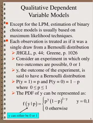
II. Introduction • Qualitative responses • A dependent variable that takes only a limited number of values • Graduate or not, promoted or not, move or stay • In this class: only two values • Also called Binary Choice Models • a) Whenever DV takes only two values
Introduction (cont.) • 3. Examples • a) What factors lead consumers to buy your company's product or service vs. not buy it? • b) What factors make some sport franchises move and others stay? • c) Why did some people vote for Obama and others vote for McCain? • d) What are the characteristics that make some people acceptable jurors and make others not acceptable?
Introduction (cont.) • 4. All of these example share a common characteristic • a) DV with only two values • (1) Buy or not buy • (2) Move vs. stay • (3) Vote for Obama vs. vote for McCain • (4) Acceptable juror vs. not acceptable
III. Everything That Follows Refers to Binary Choice Models STAY? MOVE?
IV. Do Not Use OLS • A. Model: Y = + X + • Example • 1. Y is probability that franchise moves • 2. X is attendance • 3. Although Y is probability. . . .
Do Not Use OLS (cont.) (recall: Y is probability) • 4. Y equals • a) 1 for those that move • b) 0 for those that stay • 5. Y is dummy variable
Do Not Use OLS (cont.) • Don't use OLS when Y is dummy variable because . . . • #1) parameter estimates will be inefficient because the disturbance is heteroskedastistic • #2) standard F, R2 and adj. R2incorrect • Last two involve variation in continuous DV • but DV here is discrete • #3) predicted y values could be outside 0, 1 interval • Could get negative probabilities!!
Do Not Use OLS (cont.) • 2. As stated above, there is no meaningful standard F or R2 • 3. However, we will cover how to calculate an equivalent of each
V. Overview • A. Binary choice models assume that individuals (or organizations) • 1. Are faced with TWO OUTCOMES (a choice between two alternatives or can fall into one of two categories) and • 2. where they end up depends upon observable characteristics and factors
Overview (cont.) • B. Two Main Purposes • 1. Find the relationships between • a) a set of characteristics (X) describing the individual/organization and • b) the probability of one outcome (the individual/organization will make a certain choice or fall into a certain category.) • 2. Determine the probability that an individual/organization with a given set of characteristics will fall into one outcome. • EXAMPLE: FRANCHISE MOVES
Who Uses This • Some attorneys hire consultants who help select jurors based upon the likelihood that a potential juror would be favorable to that attorney’s client. • Those consultants use binary choice models.
Who Uses This • Some loan officers use credit scoring techniques that predict whether a loan applicant is a good or bad credit risk based upon their characteristics. • They use binary choice models to predict whether the applicant will repay their loan.
Logic Underlying Model • Preview • 1. Start with model #1 • a) Z = + X + • 2. Model #2 • a) Y = + X + • b) Can observe Y but not Z • c) Y = 1 for high Z values • d) Y = 0 for low Z values
Logic Underlying Model (cont.) • A. Model: Z = + X + • 1. X observable • 2. Z unobservable/not measurable • a) Maybe desire to move
Logic Underlying Model (cont.) • 3. Use Y instead, where • a) Y = 1 if Z > some Z* • b) Y = 0 if Z some Z* • c) Z* is cutoff preference Desire to move Low High Z2 Z* Z1
Desire to move Low High Z2 Z* Z1 Logic Underlying Model (cont.) • 6. Y = 1 when • a) person’s Z > own Z* • b) high values for Z/high desire to move • 7. Y = 0 when • a) person’s Z own Z* • b) low Z values/low desire to move
Logic Underlying Model (cont.) • E. Summary • 1. Started with model #1 • a) Z = + X + • 2. Model #2 • a) Y = + X + • b) Can observe Y but not Z • c) Y = 1 for high Z values • d) Y = 0 for low Z values
Logic Underlying Model (cont.) • F. Technical Points • 1. Functional form • a) ln[P / (1 – P)] = + X + • b) where P is • (1) any value between 0 & 1 • (2) or between 0 & 100 if % form • (3) P usually interpreted as probability of event occurring
Logic Underlying Model (cont.) ln[P / (1 – P)] = + X + • c) [P / (1 – P)] • (1) odds ratio • (2) if > 0 • (a) means X rising increases ln of odds ratio • (b) most interpret as: "higher values of X increase probability of event occurring" • (c) makes sense: as P rises, odds ratio also rises • what happens to P if < 0? • What happens to P if = 0?
Logic Underlying Model (cont.) • 2. Binary choice model has two forms • a) Estimation procedure depends on the form • b) P is between 0 & 1 • (1) Maybe a % • (2) Calculate DV = ln[P / (1 – P)] • (3) Estimate by OLS • c) P is only 0 or 1 • (1) Estimate by logit method
VII. Interpreting and Using Output From Logit Regression (Logit estimation method is used when your DV is a dummy variable)
Model Estimated • DV • MOVE = 1 if franchise moved = 0 if franchise stayed • IVs: • WINPCT average winning percentage per season • PUBOWNST = 1 if team plays in mostly publicly- financed stadium or arena = 0 if not See regression output for binary choice models.
Variable Coefficient SE Coefficient Z P Constant 0.375 2.206 0.170 0.8650 WINPCT -9.15 5.232 -1.749 0.0806 PUBOWNST 3.370 1.278 2.636 0.0085 Sample Output SEE NOTE A SEE NOTE B
Sample Output (cont.) Use these values to calculate F and adj. R2 • Loglikelihood (UR)= -41.7 • Loglikelihood (R)=-60.8
Sample Output (cont.) • Note A: • Each coefficient tells the impact (positive or negative) of the associated IV on the probability that the DV will take a value of 1. • Notice, that the coefficient only tells the direction of the impact, not the numerical impact.
Note A (cont.) • EXAMPLE: WINPCT’s coefficient = -9.15. • It is negative, so the relationship between the DV and IV is negative/indirect. • As winning pct. rises (falls), the probability of a franchise moving falls (rises)
Sample Output (cont.) • Note B: • The “Z-Statistic” is the statistic that’s calculated before the p-value (probability) is calculated. This statistic and its associated p-value are used just like t-statistics in OLS regression output.
Note B (cont.) • EXAMPLE: the Z- Statistic for PUBOWNST’s coefficient is 2.636 and its p-value is .0085. • Since this value is less than 0.05, we can conclude that type of stadium/arena financing probably has an impact on the probability of a franchise moving.
Calculating The Equivalent Of An F-statistic, An R2 And An Adj. R2 For Logit Models
BACKGROUND1) You will estimate two models by logit a) Model UR: includes all of the IVs for your final model • ln LUR is the value for “Log likelihood function” on the output • b) Model R: the only IV is C • ln LR is the value for “Restricted log likelihood” on the output
Calculating Statistics (cont.) NUMBERS TO USE IN EXAMPLES: ln LUR = -41.7 (see output) ln LR = -60.8 (see output)
Calculating Statistics (cont.) Equivalent of F-statisticInterpret this statistic like the usual F-statistic.F = 2[ ln LUR - ln LR ] is distributed as chi-squared with K-1 degrees of freedom
EXAMPLE: FCalculated = FC = 2[ ln LUR - ln LR ] = 2[- 41.7 – (-60.8)] = 2[19.1] = 38.2 Here’s how you decide if your set of IVs is related to your DV: (next slide)
Calculating Statistics (cont.) • Is your set of IVs related to your dependent variable? • Look at p-value • ≤ .05? YES • < .05? NO See regression output for binary choice models: Case #1: MLB
Calculating Statistics (cont.) Pseudo-R2 statistics • Interpret these two pseudo-R2 statistics (below) like the usual unadjusted R2and adj. R2. • They don’t explain % of variation • They do indicate FIT OF MODEL
Calculating Statistics (cont.) Equivalent of R2R2 = 1 - [ ln LUR / ln LR ] EXAMPLE: 1 - [ ln LUR / ln LR ] = 1 - [-41.7 / - 60.8 ] = 0.3141** ** NOT 31.41% (not “percentage of variation explained” in binary choice models)
Calculating Statistics (cont.) Equivalent of adj. R2 n - 1adj. R2 = 1 – (1 - R2) ------- n – K where n is your sample size and K is the number of IVs in your model, excluding the intercept. (Note: “excluding the intercept.”)