Chapter 16 Qualitative and Limited Dependent Variable Models

1. Chapter 16 Qualitative and Limited Dependent Variable Models Walter R. Paczkowski Rutgers University

2. Chapter Contents • 16.1 Models with Binary Dependent Variables • 16.2 The Logit Model for Binary Choice • 16.3 Multinomial Logit • 16.4 Conditional Logit • 16.5 Ordered Choice Models • 16.6 Models for Count Data • 16.7 Limited Dependent Variables

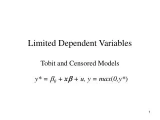
3. In this chapter, we: • Examine models that are used to describe choice behavior, and which do not have the usual continuous dependent variable • Introduce a class of models with dependent variables that are limited • They are continuous, but that their range of values is constrained in some way, and their values not completely observable • Alternatives to least squares estimation are needed since the least squares estimator is biased and inconsistent

4. 16.1 Models with Binary Dependent Variables

5. 16.1 Models with Binary Dependent Variables • Many of the choices that individuals and firms make are ‘‘either–or’’ in nature • Such choices can be represented by a binary (indicator) variable that takes the value 1 if one outcome is chosen and the value 0 otherwise • The binary variable describing a choice is the dependent variable rather than an independent variable

6. 16.1 Models with Binary Dependent Variables • Examples: • Models of why some individuals take a second or third job, and engage in ‘‘moonlighting’’ • Models of why some legislators in the U.S. House of Representatives vote for a particular bill and others do not • Models explaining why some loan applications are accepted and others are not at a large metropolitan bank • Models explaining why some individuals vote for increased spending in a school board election and others vote against • Models explaining why some female college students decide to study engineering and others do not

7. 16.1 Models with Binary Dependent Variables • We represent an individual’s choice by the indicator variable: Eq. 16.1

8. 16.1 Models with Binary Dependent Variables • If the probability that an individual drives to work is p, then P[y = 1]= p • The probability that a person uses public transportation is P[y = 0]= 1 – p • The probability function for such a binary random variable is: with Eq. 16.2

9. 16.1 Models with Binary Dependent Variables • For our analysis, define the explanatory variable as: x = (commuting time by bus - commuting time by car)

10. 16.1 Models with Binary Dependent Variables 16.1.1 The Linear Probability Model • We could model the indicator variable y using the linear model, however, there are several problems: • It implies marginal effects of changes in continuous explanatory variables are constant, which cannot be the case for a probability model • This feature also can result in predicted probabilities outside the [0, 1] interval • The linear probability model error term is heteroskedastic, so that a better estimator is generalized least squares

11. 16.1 Models with Binary Dependent Variables 16.1.1 The Linear Probability Model • In regression analysis we break the dependent variable into fixed and random parts • If we do this for the indicator variable y, we have: • Assuming that the relationship is linear: Eq. 16.3 Eq. 16.4

12. 16.1 Models with Binary Dependent Variables 16.1.1 The Linear Probability Model • The linear regression model for explaining the choice variable y is called the linear probability model: Eq. 16.5

13. 16.1 Models with Binary Dependent Variables 16.1.1 The Linear Probability Model • The probability density functions for y and e are:

14. 16.1 Models with Binary Dependent Variables 16.1.1 The Linear Probability Model • Using these values it can be shown that the variance of the error term e is: • The estimated variance of the error term is: Eq. 16.6

15. 16.1 Models with Binary Dependent Variables 16.1.1 The Linear Probability Model • We can transform the data as: • And estimate the model: by least squares to produce the feasible generalized least squares estimates • Both least squares and feasible generalized least squares are consistent estimators of the regression parameters

16. 16.1 Models with Binary Dependent Variables 16.1.1 The Linear Probability Model • If we estimate the parameters of Eq. 16.5 by least squares, we obtain the fitted model explaining the systematic portion of y • This systematic portion is p • By substituting alternative values of x,we can easily obtain values that are less than zero or greater than one Eq. 16.7

17. 16.1 Models with Binary Dependent Variables 16.1.1 The Linear Probability Model • The underlying feature that causes these problems is that the linear probability model implicitly assumes that increases in x have a constant effect on the probability of choosing to drive Eq. 16.8

18. 16.1 Models with Binary Dependent Variables 16.1.2 The Probit Model • To keep the choice probability p within the interval [0, 1], a nonlinear S-shaped relationship between x and p can be used

19. 16.1 Models with Binary Dependent Variables FIGURE 16.1 (a) Standard normal cumulative distribution function (b) Standard normal probability density function 16.1.2 The Probit Model

20. 16.1 Models with Binary Dependent Variables 16.1.2 The Probit Model • A functional relationship that is used to represent such a curve is the probit function • The probit function is related to the standard normal probability distribution: • The probit function is: Eq. 16.9

21. 16.1 Models with Binary Dependent Variables 16.1.2 The Probit Model • The probit statistical model expresses the probability p that y takes the value 1 to be: • The probit model is said to be nonlinear Eq. 16.10

22. 16.1 Models with Binary Dependent Variables 16.1.3 Interpretation of the Probit Model • We can examine the marginal effect of a one-unit change in x on the probability that y = 1 by considering the derivative: Eq. 16.11

23. 16.1 Models with Binary Dependent Variables 16.1.3 Interpretation of the Probit Model • Eq. 16.11 has the following implications: • Since Φ(β1+ β2x) is a probability density function, its value is always positive • As x changes, the value of the function Φ(β1+ β2x) changes • if β1+ β2x is large, then the probability that the individual chooses to drive is very large and close to one • Similarly if β1+ β2x is small

24. 16.1 Models with Binary Dependent Variables 16.1.3 Interpretation of the Probit Model • We estimate the probability p to be: • By comparing to a threshold value, like 0.5, we can predict choice using the rule: Eq. 16.12

25. 16.1 Models with Binary Dependent Variables 16.1.4 Maximum Likelihood Estimation of the Probit Model • The probability function for y is combined with the probit model to obtain: Eq. 16.13

26. 16.1 Models with Binary Dependent Variables 16.1.4 Maximum Likelihood Estimation of the Probit Model • If the three individuals are independently drawn, then: • The probability of observing y1 = 1, y2 = 1, and y3 = 0 is:

27. 16.1 Models with Binary Dependent Variables 16.1.4 Maximum Likelihood Estimation of the Probit Model • We now have: for x1 = 15, x2 = 6, and x3 = 7 • This function, which gives us the probability of observing the sample data, is called the likelihood function • The notation L(β1, β2) indicates that the likelihood function is a function of the unknown parameters, β1and β2 Eq. 16.14

28. 16.1 Models with Binary Dependent Variables 16.1.4 Maximum Likelihood Estimation of the Probit Model • In practice, instead of maximizing Eq. 16.14, we maximize the logarithm of Eq. 16.14, which is called the log-likelihood function: • The maximization of the log-likelihood function is easier than the maximization of Eq. 16.14 • The values that maximize the log-likelihood function also maximize the likelihood function • They are the maximum likelihood estimates Eq. 16.15

29. 16.1 Models with Binary Dependent Variables 16.1.4 Maximum Likelihood Estimation of the Probit Model • A feature of the maximum likelihood estimation procedure is that while its properties in small samples are not known, we can show that in large samples the maximum likelihood estimator is normally distributed, consistent and best, in the sense that no competing estimator has smaller variance

30. 16.1 Models with Binary Dependent Variables 16.1.5 A Transportation Example • Let DTIME = (BUSTIME-AUTOTIME)÷10, which is the commuting time differential in 10-minute increments • The probit model is: P(AUTO = 1) = Φ(β1+ β2DTIME) • The maximum likelihood estimates of the parameters are:

31. 16.1 Models with Binary Dependent Variables 16.1.5 A Transportation Example • The marginal effect of increasing public transportation time, given that travel via public transportation currently takes 20 minutes longer than auto travel is:

32. 16.1 Models with Binary Dependent Variables 16.1.5 A Transportation Example • If an individual is faced with the situation that it takes 30 minutes longer to take public transportation than to drive to work, then the estimated probability that auto transportation will be selected is: • Since 0.7983 > 0.5, we “predict” the individual will choose to drive

33. 16.1 Models with Binary Dependent Variables 16.1.6 Further Post-Estimation Analysis • Rather than evaluate the marginal effect at a specific value, or the mean value, the average marginal effect (AME) is often considered: • For our problem: • The sample standard deviation is: 0.0365 • Its minimum and maximum values are 0.0025 and 0.1153

34. 16.1 Models with Binary Dependent Variables 16.1.6 Further Post-Estimation Analysis • Consider the marginal effect: • The marginal effect function is nonlinear

35. 16.2 The Logit Model for Binary Choice

36. 16.2 The Logit Model for Binary Choice • Probit model estimation is numerically complicated because it is based on the normal distribution • A frequently used alternative to the probit model for binary choice situations is the logit model • These models differ only in the particular S-shaped curve used to constrain probabilities to the [0, 1] interval

37. 16.2 The Logit Model for Binary Choice • If L is a logistic random variable, then its probability density function is: • The cumulative distribution function for a logistic random variable is: Eq. 16.16 Eq. 16.17

38. 16.2 The Logit Model for Binary Choice • The probability p that the observed value y takes the value 1 is: Eq. 16.18

39. 16.2 The Logit Model for Binary Choice • The probability that y = 1 is: • The probability that y = 0 is:

40. 16.2 The Logit Model for Binary Choice • The shapes of the logistic and normal probability density functions are somewhat different, and maximum likelihood estimates of β1 and β2 will be different • However, the marginal probabilities and the predicted probabilities differ very little in most cases

41. 16.2 The Logit Model for Binary Choice 16.2.1 An Empirical Example from Marketing • Consider the Coke example with:

42. 16.2 The Logit Model for Binary Choice 16.2.1 An Empirical Example from Marketing • Based on ‘‘scanner’’ data on 1,140 individuals who purchased Coke or Pepsi, the probit and logit models for the choice are:

43. 16.2 The Logit Model for Binary Choice Table 16.1 Coke-Pepsi Choice Models 16.2.1 An Empirical Example from Marketing

44. 16.2 The Logit Model for Binary Choice 16.2.1 An Empirical Example from Marketing • The parameters and their estimates vary across the models and no direct comparison is very useful, but some rules of thumb exist • Roughly:

45. 16.2 The Logit Model for Binary Choice 16.2.2 Wald Hypothesis Tests • If the null hypothesis is H0: βk = c, then the test statistic using the probit model is: • The t-test is based on the Wald principle

46. 16.2 The Logit Model for Binary Choice 16.2.2 Wald Hypothesis Tests • Using the probit model, consider the two hypotheses:

47. 16.2 The Logit Model for Binary Choice 16.2.2 Wald Hypothesis Tests • To test hypothesis (1) in a linear model, we would compute: • Noting that it is a two-tail hypothesis, we reject the null hypothesis at the α = 0.05 level if t≥ 1.96 or t ≤ -1.96 • The calculated t-value is t = -2.3247, so we reject the null hypothesis • We conclude that the effects of the Coke and Pepsi displays are not of equal magnitude with opposite sign

48. 16.2 The Logit Model for Binary Choice 16.2.2 Wald Hypothesis Tests • A generalization of the Wald statistic is used to test the joint null hypothesis (2) that neither the Coke nor Pepsi display affects the probability of choosing Coke

49. 16.2 The Logit Model for Binary Choice 16.2.3 Likelihood Ratio Hypothesis Tests • When using maximum likelihood estimators, such as probit and logit, tests based on the likelihood ratio principle are generally preferred • The idea is much like the F-test • One test component is the log-likelihood function value in the unrestricted, full model (lnLU) evaluated at the maximum likelihood estimates • The second ingredient is the log-likelihood function value from the model that is ‘‘restricted’’ by imposing the condition that the null hypothesis is true (lnLR)

50. 16.2 The Logit Model for Binary Choice 16.2.3 Likelihood Ratio Hypothesis Tests • The restricted probit model is obtained by imposing the condition β3 = -β4: • We have LR = -713.6595 • The likelihood ratio test statistic value is: