Limited Dependent Variables

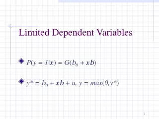
1. Limited Dependent Variables • Often there are occasions where we are interested in explaining a dependent variable that has only limited measurement • Frequently it is even dichotomous.

2. Examples • War(1) vs. no War(0) • Vote vs. no vote • Regime change vs. no change

3. These are often Probability Models • E.g. • Power disparity leads to war: • Where Yt is the occurrence (or not) of war, and Xt is a measure of power disparity • We call this a Linear Probability Model

4. Problems with LPM Regression • OLS in this case is called the Linear Probability Model • Running regression produces some problems • Errors are not distributed normally • Errors are heteroskedastic • Predicted Ys can be outside the 0.0-1. bounds required for probability

5. Logistic Model • We need a model that produces true probabilities • The Logit, or cumulative logistic distribution offers one approach. • This produces a sigmoid curve. • Look at equation under 2 conditions: • Xi = +∞ • Xi = -∞

6. Sigmoid curve

7. Probability Ratio • Note that • Where

8. Log Odds Ratio • The logit is the log of the odds ratio, and is given by: • This model gives us a coefficient that may be interpreted as a change in the weighted odds of the dependent variable

9. Estimation of Model • We estimate this with maximum likelihood • The significance tests are z statistics • We can generate a Pseudo R2 which is an attempt to measure the percent of variation of the underlying logit function explained by the independent variables • We test the full model with the Likelihood Ratio test (LR), which has a χ2 distribution with k degrees of freedom

10. Neural Networks • The alternate formulation is representative of a single-layer perceptron in an artificial neural network.

11. Probit • If we can assume that the dependent variable is actually the result of an underlying (and immeasurable) propensity or utility, we can use the cumulative normal probability function to estimate a Probit model • Also, more appropriate if the categories (or their propensities) are likely to be normally distributed • It looks just like a logit model in practice

12. The Cumulative Normal Density Function • The normal distribution is given by: • The Cumulative Normal Density Function is:

13. The Standard Normal CDF • We assume that there is an underlying threshold value (Ii) that if the case exceeds will be a 1, and 0 otherwise. • We can standardize and estimate this as

14. Probit estimates • Again, maximum likelihood estimation • Again, a Pseudo R2 • Again, a LR ratio with k degrees of freedom

15. Assumptions of Models • All Y’s are in {0,1} set • They are statistically independent • No multicollinearity • The P(Yi=1) is normal density for probit, and logistic function for logit

16. Ordered Probit • If the dependent variable can take on ordinal levels, we can extend the dichotomous Probit model to an n-chotomous, or ordered, Probit model • It simply has several threshold values estimated • Ordered logit works much the same way

17. Multinomial Logit • If our dependent variable takes on different values, but they are nominal, this is a multinomial logit model

18. Some additional info • The Modal category is good benchmark • Present % correctly predicted • This can be calculated and presented. • This, when compared to the modal category, gives us a good indication of fit.

19. Stata • Use Leadership Change data • (1992 cross section)1992-Stata

20. Test different models • Dependent variable Leadership change • Examine distribution tables ledchan1 • Independent variables • Try different • Try corr and then (pwcorr)

21. Try the following regress ledchan1 grwthgdp hlthexp illit_f polity2 logit ledchan1 grwthgdp hlthexp illit_f polity2 logistic ledchan1 grwthgdp hlthexp illit_f polity2 probit ledchan1 grwthgdp hlthexp illit_f polity2 ologit ledchan1 grwthgdp hlthexp illit_f polity2 oprobit ledchan1 grwthgdp hlthexp illit_f polity2 mlogit ledchan1 grwthgdp hlthexp illit_f polity2 tobit ledchan1 grwthgdp hlthexp illit_f polity2, ul ll

22. Tobit • Assumes a 0 value, and then a scale • E.g., the decision to incarcerate • 0 or 1 • (Imprison or not) • If Imprison, than for how many years?

23. Other models • This leads to many other models • Count models & Poisson regression • Duration/Survival/hazard models • Censoring and truncation models • Selection bias models