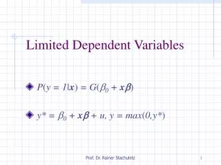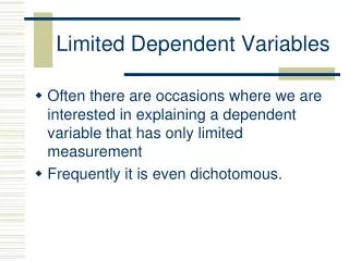
Limited Dependent Variables
Limited Dependent Variables. Poisson Model. The Poisson Regression Model. y takes on relatively few values (including zero) Number of children born to a woman Number of times someone is arrested in a year Number of patents applied for by a firm in a year

Limited Dependent Variables
E N D
Presentation Transcript
Limited Dependent Variables Poisson Model
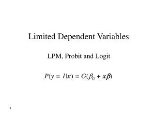
The Poisson Regression Model • y takes on relatively few values (including zero) • Number of children born to a woman • Number of times someone is arrested in a year • Number of patents applied for by a firm in a year • A linear model for E(y|x) may not provide the best fit but its always a good place to start • We start with modeling the expected value of y as E(y|x1, x2, …, xk) = exp(b1x1, b2x2,…, bkxk) • Ensures that predicted values will always be positive
Poisson Regression, cont. • So, how do we interpret coefficients in this case? • Take the logs of both sides • log(E(y|x1, x2, …, xk)) = log(exp(b1x1, b2x2,…, bkxk)) • The log of the expected value is linear • %ΔE(y|x) ≈ (100bj)Δxj • 100bj is the approximate percentage change in E(y|x) given a one unit increase in xj
Poisson Regression, cont • We can also get a more precise estimate of the effect of a change in x. The proportionate change in the expected value is: • [exp(b1x1, b2x2,…, bkx1k) / exp(b1x1, b2x2,…, bkx0k)] – 1 = exp(bkΔxk) – 1 • When xk is a dummy variable, for example, the formula becomes 100*[exp(bk) – 1] to get a percentage change
Poisson Regression, cont • Because E(y|x1, x2, …, xk) = exp(b1x1, b2x2,…, bkxk) is nonlinear in its parameters, we cannot use OLS to estimate this equation • Instead we will rely on quasi-maximum likelihood estimation • Recall that we have been using normality as the standard distributional assumption for linear regression • A count variable cannot have a normal distribution, particularly when it takes on very few values (binary variable is the extreme case)
Poisson Regression, cont • Instead we will use a Poisson distribution • The Poisson distribution is entirely determined by its mean • P(y = h|x) = exp[-exp(xb)][exp(xb)]h / h! • This distribution allows us to find conditional probabilities for any values of the explanatory variables. • For example: P(y = 0|x) = exp[-exp(xb)]. Once we have the estimates of the bjs, we can plug them into the probabilities for various values of x. • We form the log likelihood and maximize • L(b) = Σli (b) = Σ{yixib – exp(xib)}
Poisson Regression, cont • As with other nonlinear methods, we cannot directly compare the magnitudes of the estimated coefficients with OLS estimates, they have to first be multiplied by a factor: • ∂E(y|x1,x2,x3,..xk)/∂xj = bj exp(b0+ b1x1+ b2x2+..+ bkxk)
Poisson Regression, cont • The Poisson distribution has a nice robustness property: whether or not the Poisson distribution holds we still get consistent, asymptotically normal estimators of the bj. • The characteristics of the Poisson distribution are very restrictive—all higher moments are determined entirely by the mean • Var(y|x) = E(y|x) • There is a simple correction we can make to the standard errors when we assume that the variance is proportional to the mean • Var(y|x) = σ2E(y|x) where σ2is an unknown parameter
Poisson Regression, cont • When σ2 = 1, we have the Poisson assumption • When σ2 >1, the variance is greater than the mean for all x—this is called overdispersion • It is easy to adjust the usual Poisson MLE standard errors. • Define ûi = yi – ŷi • A consistent estimator of σ2 is (n – k – 1) -1Σ(û2i / ŷi) • Multiply the standard errors by σ^ • Stata Example 10-1