Download
1 / 94
960 likes | 1.18k Vues
An Overview of the NCEP Eta Model. COMET/UCAR SOO Symposium on NWP. 28 March 2000. Presented by Thomas Black. EMC/Mesoscale Modeling Branch. EDAS slides by Eric Rogers. Outline. Brief model description Eta Data Assimilation System Physics Examples of products/statistics Future. Domain.

E N D
An Overview of the NCEP Eta Model COMET/UCAR SOO Symposium on NWP 28 March 2000 Presented by Thomas Black EMC/Mesoscale Modeling Branch EDAS slides by Eric Rogers
Outline • Brief model description • Eta Data Assimilation System • Physics • Examples of products/statistics • Future
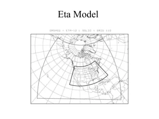
Domain • Semi-staggered Arakawa E grid • 32km horizontal resolution • 45 vertical eta layers • Silhouette step topography
32km Domain Topography w/ Water Points
32km CONUS Topography w/ Water Points
ground ground Sigma and Eta Coordinates P P MSL is small At point P: At point P: is small
Eta Coordinate Reference heights and temperatures taken from the standard atmosphere P= LM-3 PMSL LM-3 LM-2 P= LM-2 PMSL Z= ZREF at P = LM-2 PSMSL P= LM-1 PMSL LM-1 Z= ZREF at P = LM-1 PSMSL Z=0 LM=1 P=PMSL Mean Sea Level
Eta Model 45-Layer Distribution 25 hPa 27 hPa 29 29 27 26 26 24 23 250 hPa 24 26 30 31 32 32 32 33 500 hPa 33 33 33 33 32 31 29 700 hPa 27 23 21 19 18 18 17 850 hPa 16 14 13 13 13 13 12 12 12 1000 hPa 12 11 8 6 5 2
H H H V V d d H H V V V H H H V V H H V V V H H H V V The Semi-Staggered E Grid H mass point V velocity point constant transformed latitude constant transformed longitude
Eta Data Assimilation System GOAL : Produce best possible initial conditions for the Eta Model forecast* • KEY COMPONENTS - State of the art analysis (variational) - Consistency between assimilating and forecast model (resolution, physics, dynamics) - Intelligent selection and use of observations * NOT necessarily the same as fitting all the observations exactly
What is 3D-VAR? • An analysis technique that attempts to minimize analysis error • Takes background (forecast) and observation error into account • Variational method allows use of “non-traditional” data sources, such as GOES precipitable water
- Stream function - Temperature - Potential function - Specific humidity - Surface pressure - Geopotential height ETA 3DVAR ANALYSIS (Parrish et al. 1996 NWP Preprint Volume) • Loosely patterned after NCEP global SSI analysis • Analysis variables: • More adaptable than OI for using new data types (e.g., NEXRAD radial velocities used in Eta-10 runs during 1996 Olympics)
EDAS Original Configuration Eta-48 fcst 00Z/12Z Eta-29 fcst 03Z/15Z
WHY DO CYCLING? • Initial conditions more consistent with forecast model • Less spinup of divergence, cloud, precipitation, and TKE • More accurate representation of soil moisture
Observations Used By ETA 3DVAR • Upper air data - Rawinsonde height/temperature/wind/moisture - Dropwindsondes - Wind Profilers - NESDIS thickness retrievals from polar orbiting satellites (oceans only) - VAD winds from NEXRAD - Aircraft (conventional and ACARS) winds/temps - Satellite cloud drift winds - SSM/I and GOES precipitable water retrievals - Synthetic tropical cyclone data • Surface data - Surface land wind/temperature/moisture - Ships and buoys - SSM/I oceanic surface winds
DATA QUALITY CONTROL • CQC: Complex QC of raob height/temps (baseline, hydrostatic, lapse rate, radiation correction, etc.) • ACQC : Quality control of conventional aircraft data (remove duplicates, track checks, create “superobs”) • SDMEDIT : NCEP Senior Duty Meteorologist can flag all or parts of suspect raobs • 3DVAR : Analysis performs gross check vs. first guess: - Temperature : +/- 15oC - Wind :+/- 25 ms-1 - RH : +/- 90% - Precipitable water : +/- 12 g/kg - Height : +/- 100 m
Use of Surface Data: Eta OI vs. Eta 3DVAR Eta OI Analysis Eta 3DVAR Analysis
New 3DVAR tested in July 1998 and showed improved fit to surface and raobs (especially moisture) • Re-tuned 3DVAR implemented on 3 November 1998 • We thought everything was OK….. BUT……..
24-H ACCUMULATED PRECIPITATION EQUITABLE THREAT SCORES: ALL FCSTS Solid = Eta Short Dash = NGM Long Dash = AVN/MRF 12/1/97 - 2/28/98 12/1/98 - 2/28/99 10-15% drop in Eta skill between 1997-98 and 1998-99
Persistent synoptic error in Eta-32 during winter of 98-99: weaker and faster Eastern Pacific troughs/cyclones than observed Example : 48-h Forecasts valid 1200 UTC 17 March 1999
PROBLEM 1: November 98 change degraded mass/wind balance in 3DVAR • If mass / wind balance well-behaved, positive height correction is coincident with center of anticyclonic wind correction 850 mb ANL-GUESS height/wind 80KM EDAS valid 00Z 3/15/99 • Note 10 degree longitude displacement between centers of wind and height correction • Problem is most severe in regions and at analysis times without widespread raob data but with large amounts of wind or mass only data (e.g., satellite winds)
SOLUTION : Improve geostrophic coupling of mass/wind analysis corrections in 3DVAR (5/99) Original 3DVAR analysis Improved 3DVAR analysis Note: Improved height/wind coupling near Aleutians
PROBLEM 2: Horizontal/vertical correlations too narrow : observation had VERY limited impact on analysis away from its level SOLUTION: Expand the influence of the observations (5/99) • One observation test : Insert one height observation 10 m greater than first guess at 200, 500, 900 mb and measure impact in horizontal/vertical
Original 32-km 3DVAR Improved 32-km 3DVAR 200 mb 900 mb
Performance of new 3DVAR : 3 December 1998 to 16 January 1999 test at 80 km resolution 24-h accumulated precipitation threat scores: All forecasts Dashed = Modified 3DVAR Solid = Operational 3DVAR Equitable Threat Score Threshold (in)
The Forecast Model Split Explicit Integration: Dynamics • Fundamental prognostic variables • T, u, v, q, Psfc, TKE, cloud water/ice • Inertial gravity wave adjustment • forward-backward scheme (Dt=90s) • Vertical advection • Euler-backward scheme • centered in space • piecewise linear for q
Split Explicit Integration: Dynamics • Horizontal advection • modified Euler-backward scheme • Janjic advection in space • conservative, (nearly) shape-preserving scheme for H20 • upstream advection near boundaries
Split Explicit Integration: Physics • Betts-Miller-Janjic convection • Mellor-Yamada level 2.5 turbulent exchange • GFDL radiation • explicit cloud water/ice prediction • 4-layer NOAH land surface package • D2 horizontal diffusion
One-wayBoundary Conditions • 3-hour tendencies • 6 hour old AVN forecast used
vertical advection 1 5 Runstream Schematic of Eta Model Integration gridscale cloud gridscale precip convection turbulence horizontal advection inertial grv wave adjustment 1 2 3 4 5 6 7 8 9 1 0 1 1 1 2 1 3 1 4 1 6 timestep t = 90 s Radiative temperature tendency updates Shortwave: 40 timesteps (1 hour) Longwave: 80 timesteps (2 hours)
The Betts-Miller-Janji Convection Scheme in the Eta Model References: Betts, 1986 (QJRMS) Betts and Miller, 1986 (QJRMS) Janji, 1994 (MWR) • Deep (precipitating) convection • Temperature reference profile • Moisture reference profile • Convective adjustment • Modification for “precipitation efficiency” • Shallow (non-precipitating) convection • Temperature reference profile • Moisture reference profile
Find the Deep Convective Clouds 1. For all ‘parcels’ within 0.2xPsfc mb of the ground find Psat andES 2. At each point, select parcel with the maximum ES 3. Given Psat, choose cloud base as the model level just below it 4. Adjust cloud base if needed: (a) at least 25 mb above middle of lowest layer (b) at least one model layer above lowest layer 5. Compute Tmad above cloud base using ES and P in lookup tables 6. Set cloud top at highest level where Tmad<T-T (currently T=0) 7. Gather all clouds at least 0.2xPsfc mb deep
1. Define ‘deficit from saturation pressure’ (DSP) for cloud bottom, freezing level, and cloud top (larger DSPdrier state) Construction of 1st Guess Humidity Reference Profile For Deep Convection 2. Linearly interpolate DSP’s for values between these 3 levels 3. Define the reference humidity profile as qsat in each layer
The Enthalpy Correction Modify the profiles to ensure enthalpy in the cloud column is conserved during adjustment Initially: Corrections: Currently the above procedure is repeated two times
1. Relax model profiles of T and q toward the reference profiles where relaxation time equals 2400 s Final Deep Convective Adjustment 2. Convective rainfall amount is 3. At any point, deep adjustment is ignored and a “swap” to shallow convection occurs if: (a) S < 0 (b) precipitation is negative
Deep Convective Adjustment of Temperature Upward Transport of Heat cloud top REFERENCE TEMPERATURE AMBIENT TEMPERATURE cloud base
Modification for ‘Precipitation Efficiency’ Examination of Eta integrations shows: As convective precipitation increases, entropy changes decrease. So defineprecipitation efficiencyas the ratio: Numerator: Q arising from entropy change Denominator: Q arising from precipitation (H=0)
Thus, larger E less mature system smaller E more mature system USE E TO MODERATE HEAVY RAIN IN LONG-LIVED MATURE SYSTEMS (A) Modify the humidity reference profile (B) Modify the relaxation time
Humidity Reference Profile Limits q cloud top HUMIDITY REFERENCE PROFILE E=0.2 E=1 MOISTPROFILELIMIT p DRY PROFILE LIMIT cloud base DSP’s vary between DRY (fast) and MOIST (slow) limits
Top -1875 Pa Freezing -5875 Pa Bottom -3875 Pa Values of DSP Limits Dry limits MOIST DSP limits equal 0.85 times DRY limits. Att=0, DSP’s are set to the DRY limits.
Modification of Relaxation Time Multiply the standard change due to adjustment by some quantity F which is a function of the precipitation efficiency OR For simplicity assume F is linear. Then empirically: 0.7 <F< 1.0 for 0.2 <E< 1.0
Find the Shallow Convective Clouds 1. Find the tops of the “swapped” clouds (a) set a preliminary top at pbot - 0.2xPsfc mb (pbot > 450 mb) (b) reset top to level where maximum (RH)/p occurs 2. Gather all clouds that are: (a) greater than 10 mb deep (b) less than 0.2xPsfc mb deep (c) at least two model layers deep
(cpT p) = 0 Correct Tref assuming Construction of Temperature Reference Profile For Shallow Convection cloud top Mixing Line REFERENCE TEMPERATURE cloud base