Applications Statistical Graphical Models in Music Informatics
360 likes | 534 Vues
I548 Presentation. Applications Statistical Graphical Models in Music Informatics. Yushen Han Feb 10 2011. Statistical Graphical Models. graph-based representation for a probabilistic distribution in high-dimensional space while specifying conditional independence structure

Applications Statistical Graphical Models in Music Informatics
E N D
Presentation Transcript
I548 Presentation Applications Statistical Graphical Models in Music Informatics Yushen Han Feb 10 2011
Statistical Graphical Models • graph-based representation for a probabilistic distribution in high-dimensional space while specifying conditional independence structure • directed acyclic graph(DAG) - Bayesian Network • undirected graph(UG)- Markov Random Field • Mixed graph
Markov Condition on a Bayesian Network probabilistic distribution High-dimensional space Conditional independence From www.eecs.berkeley.edu/ewainwrig/ Markov Condition: XA and XB are conditionally independent given XS whenever S separates A and B
Musical Application: Bayesian Identification of Chord from Audio mode key octave root Attributes Chroma (pitch-class) tuning Observation: Peak frequencies and corresponding amplitude factorization of the joint by Bayesian Inference
Application I: Score Following/Alignment Music score (given) Score Following: Online (real time) Score Alignment: Offline (no need to be in real time) Performance audio of this piece (given) Establishing a correspondence between the two above
Application I: Score Following Best “guess” of the current location given what the computer had heard SINCE THE BEGINNING UP TO THE MOMENT
Observation - “Frames” of Audio Audio (waveform) Spectrogram (via Short-time Fourier transform)
Score Following • Difficulties • Tempo rubato (expressive and rhythmic freedom) • Pitch / amplitude vibrato ( ) • Polyphony music • Noise • (occasional) wrong notes etc. • Realtime computational requirement • Solutions • Assuming tempo change is smooth (mostly desirable) • Robust probabilistic data model on normalized semigram • Training to learn a prior (e.g. note length distribution) • Optimized particle filtering for 2-D State-space model
Proposed Solution with 2-D State-space Model (Bayesian Network) • Assuming smooth tempo change for tempo rubato • Two-dimensional state-space model • Proposing a unit of tempi: • S(t) - Musical time elapse per audio frame at frame t • Interpretation: during one audio frame of fixed length (roughly 64ms, 512 samples at 8000Hz sampling rate), how much musical time (in terms of 1/384 notes) is elapsing • In another word, how much of the score the performer covers every 64ms (not precisely the conventional tempo)
2-D State-space Model Current “speed” at this frame Accumulative “speed” up to this frame –location State variables in one audio frame (notice conditional independence) 0.64ms 0.64ms
Physical Analogy – Integration of the Speed speed 1 1 1 1 3 1 4 location 2
Physical Analogy – Integration of the Speedwith stochastic components speed 1.0 0.95 1.1 1.05 Speed fluctuation 2.12 3.19 1.0 4.11 location Observation error also involved
Physical Analogy - to make a tractable problem Assuming discrete state transition with {-0.1, -0.05, 0, 0.05, 0.1} with prob distribution {0.1, 0.2, 0.4 ,0.2, 0.1} for smoothness. speed 1.0 0.95 1.1 1.05 Speed fluctuation 2.12 3.19 1.0 4.11 location Observation error also involved Assuming Gaussian noise in observation
Relationship to Kalman Filter • Particle filtering • (Using White board)
Score Following – Data Model • Data model using semigram • Regarding discretized observation as a histogram Chord template (pre-learned)
Score Following – Demo in R • Data model in R • Visualization of results in XCode
Application II:Graph Model to Estimate Expert Pianists’ Perceptual Present- with the help of audio-score alignment technique
Background • Curtain eras of classical music – no improvisation, no wrong notes etc. • For a certain piece of music, performance varies in tempo, dynamic, articulation, vibrato etc. , depending on the interpretation of the performer • (This research) focuses on the tempo change of piano music
Chopin Mazurka Op. 30, No.2 Rubinstein Horowitz Michelangeli http://www.youtube.com/watch?v=PjYV7lJezvc http://www.youtube.com/watch?v=vGAQONeLnXk http://www.youtube.com/watch?v=qJmaz1OEGTU
Motivation • Musical Perceptual Present • Recent studies in diverse fields of inquiry, including music philosophy and psychology, lend converging evidence that musical attention of both performers and listeners is primarily focused successively small “chunks” of material (hypothetically 2–10 seconds in the past) rather than larger formal relationships.
Motivation • Instead of individual style, we are in search of a “common interpretation” shared among a collection of expert pianists • Focus purely on tempo change per beat (since the attack of piano note is easy to capture).
Data • Human corrected accumulative time per beat which is equivalent to IBI Inter Beat Interval • N = 32 performances ( include different performances of the same pianist ) • For the existence of the MLE, we proceed a small chunk of data at a time I = { 7, 8, 9, 10 }
Data cont. - preprocessing • # !!!performance-id: pid9062-19 • # !!!title: Mazurka in B minor, Op. 30, No. 2 • # !!!trials: 1 • # !!!date: 2007/02/15/ • # !!!reverse-conductor: Craig Stuart Sapp • # !!!performer: IdilBiret • # !!!performance-date: 1990 • # !!!label: Naxos 8.550359 • # !!!label-title: Chopin: Mazurkas (Complete) • # !!!offset: 0 • 0.578 0:3 • 1.398 1:1 • 1.708 1:2 • 2.228 1:3 • 2.668 2:1 • 3.088 2:2 • 3.748 2:3 • 4.336 3:1 • 4.588 3:2 • 4.998 3:3 • 5.498 4:1 • 5.828 4:2 • 6.428 4:3 • 7.028 5:1 • 7.355 5:2 • 7.968 5:3 • 8.428 6:1 • 8.838 6:2 • 9.418 6:3 • 9.878 7:1 • 10.158 7:2 • 10.678 7:3 • 0.720 • 0.855 • 0.745 • 0.800 • 0.490 • 0.610 • 0.530 • 0.540 • 0.550 • 0.540 • 0.530 • 0.570 • … • 0.135 • -0.110 • 0.055 • -0.310 • 0.120 • -0.080 • 0.010 • 0.010 • -0.010 • … Original Data: Accumulative time per beat IBI difference between beats InterBeatInterval (IBI)
Data cont. - preprocessing • “Normalization” • Since the overall duration of each performance varies significantly E.g. Mazurka Op. 30. No. 2 Sec. Performance index We “stretch” the overall duration of each performance to line up with the median of all performances - can be problematic
Model • For each “trunk” of timing data X of I dimensions (beats) across N performances: • N performances are considered i.i.d. repetitions • we assume: X ~ Ν( 0, Σ ) • where the difference in IBI equals to 0 suggests that the tempo is nearly constant “on average” (of course, but could be problematic) • We study the structure of I by I covariance matrix Σ • Can obtain an estimate of
Model cont. – check the normality • See the movie in R
Graph Models • A toy example for I = 4 case -> 3 hypotheses • H: Fully saturated model (I-1=3 order Markov chain) diff. IBI • H0: A smaller model (I-2=2 order Markov chain) • H00: The smallest model (I-3=1 order Markov chain)
Graph Models cont. • What does this graph mean? • Conditional Independence!
Graph Models cont. • Conditional independence in the graph suggests different structures in the covariance matrix To apply reconstruction algorithm
Graph Models cont. - Testing • Testing each pair of hypotheses -2Log(Q) ~ • Accepting the result only when every single pair of hypotheses of the smallest difference between the alternative and the null hypotheses are not rejected (as small step as possible) • Apply an appropriate degree of freedom ( = difference in number of edges between 2 graphs )
Results - Testing • See R plot
Results – Interpretation • “smoothed” results by using a sliding window of different lengths • A “voting” mechanism • Room to interpret …
Results – Interpretation “smoothed” results by using a sliding window of different lengths
Results – Interpretation “smoothed” results by using a sliding window of different lengths
Results – Interpretation Using “anchor points” to summarize the results
