Download
1 / 7
130 likes | 413 Vues
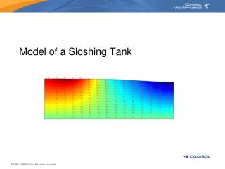
Model of a Sloshing Tank. Background. Oil tankers and transport trucks are two examples where sloshing can occur within a tank. If sloshing is too extreme, it can create a non-uniform distribution of weight within the tank.

E N D
Background • Oil tankers and transport trucks are two examples where sloshing can occur within a tank. • If sloshing is too extreme, it can create a non-uniform distribution of weight within the tank. • This model is a demo of free surface flow modeling using the Moving Mesh user-interface available in COMSOL Multiphysics • The method used to move and deform the mesh in COMSOL Multiphysics is known as an Arbitray Lagrangian Eulerian (ALE) method • The equations solved are the Navier-Stokes equations in a moving reference frame defined by the moving mesh
Model Definition • The free surface condition (no flow cross the surface boundary) is formulated with the built in tangent and normal coordinate system boundary conditions for the moving mesh, and a neutral-stress boundary condition for Navier-Stokes equations at the top surface. • Surface tension effects are neglected in this example, but could be included if needed • The flow, initially at rest, is driven by an oscillating gravity vector. This is to mimic a periodic ’tank’ motion. This can be visualized using a deformation plot, where the entire frame is deformed according to the gravity vector. • The example is made in 2D but could be generalized to 3D – you would only need a computer with more RAM compared to the 2D case.
Model Definition • The fluid is glycerol with: • h = 1.49 Ns/m2 • r = 1270 kg/m3 • The walls of the ’tank’ allow free slip. • The gravity vector is (g_x,g_y)T, with: g_x = g*sin(phi_0*sin(2*pi*f*t)), g_y = -g*cos(phi_0*sin(2*pi*f*t)), g = 9.81 m/s2 phi_0 = pi/128 f = 1 s-1
Model Definition – Mesh Movie** set in presentation mode to view • The mesh deformation is computed according to the Navier-Stokes equations with the applied gravity load. • Note that higher-order finite elements are used not only within the tank to represent the flow field but also to track the free fluid surface.
Results - Movie** set in presentation mode to view • Results showing the vertical fluid velocity (y-velocty) in colors and the x-y velocity as arrows. • The internal viscous force is the only energy dissipation mechanism in this example, therefore the wave amplitude is increasing and becomes large. • After a while higher-order modes of oscillation become visible.
Results • The wave height at the right side wall