Download
1 / 73
730 likes | 962 Vues
Climate Change and Biome Shifts in Alaska and Western Canada. Current Results and Modeling Options December 2010. Participants. Scenarios Network for Alaska Planning (SNAP), University of Alaska Fairbanks EWHALE lab, Institute of Arctic Biology, University of Alaska Fairbanks

E N D
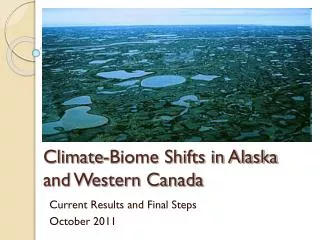
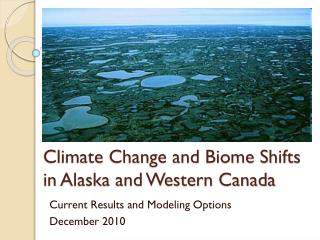
Climate Change and Biome Shifts in Alaska and Western Canada Current Results and Modeling Options December 2010
Participants • Scenarios Network for Alaska Planning (SNAP), University of Alaska Fairbanks • EWHALE lab, Institute of Arctic Biology, University of Alaska Fairbanks • US Fish and Wildlife Service • The Nature Conservancy • Ducks Unlimited Canada • Government of the Northwest Territories • Government of Canada • Other invited experts
Goals of this meeting • Review Project Goals • Summary of project background • Explanation of modeling methods and data • Update on progress thus far • Discussion and decisions from group: • Confirm clustering inputs (24 predictor variables) • Confirm resolution for clustering and re-projection (CRU vs PRISM) • Select number of clusters (15-20) • Select land cover comparisons, data and methods • Choose future decades to model • Confirm emissions scenarios (A1B, A2, B1) • Discuss data delivery and formats • Other issues? • Review Project timeline
Overview • This project is intended to: • a) develop climate and vegetation based biomes for Alaska, the Yukon and the Northwest Territories based on data, and • b) based on the climate data, identify areas that are least likely to change and those that are most likely to change over the next 100 years. • This project builds ,and makes use of, work previously conducted by SNAP, EWHALE, USFWS, TNC, and other partners. • The completed analysis will be used by partners involved in protected areas, land use, and sustainable land use planning, e.g. connectivity.
Overall objectives • Develop climate and vegetation based biomes (based on cluster analysis) for AK, Yukon, NWT, and areas to the south that may represent future climatic conditions for AK,Yukon or NWT. • Model potential climate-induced biome shift. • Based on model results, identify areas that are least or most likely to change over the next 10-90 years. • Provide maps, data, and a written report summarizing, supporting, and displaying these findings.
The Scenarios Network for Alaska and Arctic Planning (SNAP) • SNAP is a collaborative network of the University of Alaska, state, federal, and local agencies, NGOs, and industry partners. • Its mission is to provide timely access to scenarios of future conditions in Alaska for more effective planning by decision-makers, communities, and industry.
SNAP uses data for 5 of 15 models that performed best for Alaska and northern latitudes PRISM downscaled to 2 km resolution OR CRU downscaled to 10 minutes (18.4 km) Monthly temp and precip from 1900 to 2100 (historical CRU + projected) 5 models x 3 emission scenarios Available as maps, graphs, charts, raw data On line, downloadable, in Google Earth, or in printable formats No data yet: Extreme events Snowpack Coastal/Oceans SNAP Projections: based on IPCC models
Phase I: Alaska modelMapped shifts in potential biomes based on current climate envelopes for six Alaskan biomes and six Canadian Ecozones 8 http://geogratis.cgdi.gc.ca/geogratis/en/collection/detail.do?id=4361
Phase I Results:Potential Change: Current - 2100(Noting that actual species shifts lag behind climate shifts)
Improvements over Phase I • Extend scope to northwestern Canada • Use all 12 months of data, not just 2 • Eliminate pre-defined biome/ecozone categories in favor of model-defined groupings (clusters) • Eliminates false line at US/Canada border • Creates groups with greatest degree of intra-group and inter-group dissimilarity • Gets around the problem of imperfect mapping of vegetation and ecosystem types • Allows for comparison and/or validation against existing maps of vegetation and ecosystems
Cluster analysis • Cluster analysis is the assignment of a set of observations into subsets so that observations in the same cluster are similar in some sense. • Clustering is a method of “unsupervised learning” (the model teaches itself, and finds the major breaks) • Clustering is common for statistical data analysis used in many fields • The choice of which clusters to merge or split is determined by a linkage criterion (distance metrics), which is a function of the pairwise distances between observations. • Cutting the tree at a given height will give a clustering at a selected precision.
Step 1: Create a Dissimilarity Matrix • Distance measure determines how the similarity of two elements is calculated. • Some elements may be close to one another according to one distance and farther away according to another. • In our modeling efforts, all 24 variables are given equal weight, and all distances are calculated in “24-dimensional space” using RandomForest (similarity matrix, proximity matrix, distance matrix get converted into each other) Taxicab geometry versus Euclidean distance: The red, blue, and yellow lines have the same length in taxicab geometry for the same route. In Euclidean geometry, the green line has length 6×√2 ≈ 8.48, and is the unique shortest path.
Methods: Partitioning Around Medoids (PAM) • The dissimilarity matrix describes pairwise distinction between objects. • The algorithm PAM computes representative objects, called medoids whose average dissimilarity to all the objects in the cluster is minimal • Each object of the data set is assigned to the nearest medoid. • PAM is more robust than the well-known kmeans algorithm, because it minimizes a sum of dissimilarities instead of a sum of squared Euclidean distances, thereby reducing the influence of outliers. • PAM is a standard procedure
Clustering limitations • PAM must compare every data point to every other data point in the dissimilarity matrix (created by RandomForest), and create medoids • Adding additional data points affects processing requirements exponentially • Thus, in creating clusters, we were limited to approximately 20,000 data points, a fraction of the possible samples. • Total area is approximately 19 million square kilometers • This meant selecting one data point for approximately every 20 km by 20 km
Resolution limitations Data are not available at the same resolution for the entire area • for Alaska, Yukon, and BC, SNAP uses 1961-1990 climatologies from PRISM, at 2 km, • for all other regions of Canada SNAP uses climatologies for the same time period from CRU, at 10 minutes lat/long (~18.4 km) • In clustering these data, both the difference in scale and the difference in gridding algorithms led to artificial incongruities across boundaries. • One solution to both resolution and clustering limitations is to cluster across the whole region using CRU data, which is available for the entire area.
Re-Sampling to overcome AK & Can differences (=> as it applies to many GIS datasets) Different Pixel Resolutions
Re-Sampling to overcome AK & Can differences (=> as it applies to many GIS datasets) Different Pixel Resolutions resolved….
PRISM data • Unlike other statistical methods in use today, PRISM was written by a meteorologist specifically to address climate • Moving-window regression of climate vs. elevation for each grid cell • Uses nearby station observations • Spatial climate knowledge base weights stations in the regression function by their physiographic similarity to the target grid cell • PRISM is well-suited to mountainous regions, because the effects of terrain on climate play a central role in the model's conceptual framework • The primary effect of orography on a given mountain slope is to cause precipitation to vary strongly with elevation. • The topographic facet is an important climatic unit and elevation is a primary driver of climate patterns • PRISM quality depends on DEM
PRISM: 5 clusters Note: colors on all the following cluster maps are arbitrary, and are chosen merely to be distinct from one another. Coastal vs interior, northern vs southern
PRISM: 10 clusters Aleutians and coastal rainforest become distinct
PRISM: 15 clusters Latitudinal patterns in AK and BC
PRISM: 20 clusters Highest points of Brooks Range separate from coastal plain and lower foothills How many clusters can be justified?
CRU data • The station climate statistics were interpolated using thin-plate smoothing splines (ANUSPLIN) • Trivariate thin-plate spline surfaces were fitted as functions of latitude, longitude and elevation to the station data • The inclusion of elevation as a co-predictor adds considerable skill to the interpolation, enabling topographic controls on climate • Local topographic effects such as rain shadows cannot be resolved unless: (1) a predictor that is a proxy for this influence is incorporated in the interpolation, and/or (2) there are sufficient stations to capture this local dependency as a function of latitude, longitude and elevation. • In regions with sparse data, the station networks used to create these data sets are clearly unable to capture this sort of detail
CRU data alone: 5 clusters Strong latitudinal banding
CRU data alone: 10 clusters Weather station anomaly?
CRU data alone: 15 clusters Latitudinal banding persists, but more variability and east/west break
CRU data alone: 20 clusters How many clusters can be justified?
Re-projecting CRU clusters to PRISM • CRU is available for entire study area, and offers a good fit at a broader scale • PRISM offers a better fit at fine scales, with better accuracy re altitude but is not fully available for the study area • Best of both: • Cluster results from CRU data were used to train an RF classification model. • RF then classified the full PRISM datasets (where available) according to these clusters • This referred as DOWNSCALING
Comparison of results using various methods The following results were derived from the following clustering and downscaling groups: • Created clusters using 15km sample of 2km PRISM data, and downscaled to the full PRISM dataset at 2km resolution over AK, YT, BC. • Created clusters using 20km sample of 10min CRU data, and downscaled using the 2km PRISM data over AK, YT, BC.
Comparison of results: 5 clusters Trained to PRISM data, and re-projected to PRISM Trained to CRU, re-projected to PRISM data
Comparison of results: 10 clusters Trained to PRISM data Trained to PRISM data, and re-projected to PRISM Trained to CRU, re-projected to PRISM data
Comparison of results: 15 clusters Trained to PRISM data Trained to PRISM data, and re-projected to PRISM Trained to CRU, re-projected to PRISM data
Comparison of results: 20 clusters Trained to PRISM data Trained to PRISM data, and re-projected to PRISM Trained to CRU, re-projected to PRISM data
Assessing the clusters • Box plots • Congruence with existing land cover classification by modal values • Congruence with land cover classification by percent • Other metrics?
January precipitation January temperature February precipitation February temperature
July precipitation July temperature October precipitation October temperature
Landcover in Alaska and Canada Viereck Nowacki Canadian Ecoregions NLDC Landfire LANDSAT AVHRR MODIS NDVI Greenness North America Landcover
15 Cluster Solution (10min CRU) With Most Common AVHRR Landcover Class Displayed Within Each Cluster Area The logic here is that each cluster has the mode response displayed within it using a “winner-take-all” methodology AVHRR_LC 1 - Evergreen Needleleaf Forest 6 - Woodland 8 - Closed Shrubland 9 - Open Shrubland 10 - Grassland
How Pure Are These New Clusters with Regard to AVHRR Landcover?
Boreal Cordillera Boreal PLain Boreal Shield Hudson Plain Montane Cordillera Northern Arctic Pacific Maritime Prairie Southern Arctic Taiga Cordillera Taiga Plain Taiga Shield Canada Ecozones
How Pure Are These New Clusters with Regard to Canada’s Ecozones?
Boreal Cordillera Boreal PLain Boreal Shield Hudson Plain Montane Cordillera Northern Arctic Pacific Maritime Prairie Southern Arctic Taiga Cordillera Taiga Plain Taiga Shield Canada Ecozones – With 15 Cluster Solution Polygons Overlaid “Winner-take-all” Type of Mode Reclassification
Northern Arctic Southern Arctic Taiga Plain Taiga Sheild Boreal Sheild Boreal Plain Prairie Taiga Cordillera Boreal Cordillera Pacific Maritime Montane Cordillera 15 Cluster Solution with Mode Response From Canada Ecozones as Identifier of New Clusters – With Canada Ecozones Polygons Overlaid “Winner-take-all” Type of Mode Reclassification
LEVEL_2 Alaska Range Transition Aleutian Meadows Arctic Tundra Bering Taiga Bering Tundra Coast Mountains Transition Coastal Rainforests Intermontane Boreal Pacific Mountains Transition Alaska Ecoregions - Nowacki
Alaska Range Transition Aleutian Meadows Arctic Tundra Bering Taiga No MODE Value Coastal Rainforests Intermontane Boreal Pacific Mountains Transition 15 Cluster Solution Mode Response of Alaska Ecoregions – Nowacki [Level 2]
How Pure Are These New Clusters with Regard to Alaska Ecoregions (Nowacki)?
15 Cluster Solution of Alaska Ecoregions – With Nowacki [Level 2] Ecoregions Polygons Overlaid