Next Semester
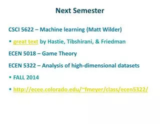
Next Semester. CSCI 5622 – Machine learning (Matt Wilder) great text by Hastie, Tibshirani , & Friedman ECEN 5018 – Game Theory ECEN 5322 – Analysis of high-dimensional datasets FALL 2014 http://ecee.colorado.edu/~fmeyer/class/ecen5322/. Project. Assignments 8 and 9

Next Semester
E N D
Presentation Transcript
Next Semester • CSCI 5622 – Machine learning (Matt Wilder) • great text by Hastie, Tibshirani, & Friedman • ECEN 5018 – Game Theory • ECEN 5322 – Analysis of high-dimensional datasets • FALL 2014 • http://ecee.colorado.edu/~fmeyer/class/ecen5322/
Project Assignments 8 and 9 Your own project or my ‘student modeling’ project Individual or team
Battleship Game • link to game
Data set 51 students 179 unique problems 4223 total problems ~ 15 hr of student usage
Bayesian Knowledge Tracing • Students are learning a new skill (knowledge component) with a computerized tutoring system • E.g., manipulation of algebra equations • Students are given a series of problemsto solve. • Solution is either correct or incorrect. • E.g., 0 0 1 0 0 1 1 0 0 0 0 0 1 0 0 0 1 1 0 1 0 1 1 1 • Goal • Infer when learning has taken place • (Larger goal is to use this prediction to make inferences about other aspects of student performance, such as retention over time and generalization to other skills)
All Or Nothing Learning Model(Atkinson, 1960s) • Two state finite-state machine Just learned Don’t Know Know Just forgotten c0 c1
Bayesian Knowledge TracingAssumes No Forgetting • Very sensible, given that sequence of problems is all within a single session. Just learned Don’t Know Know ρ0 ρ1
Inference Problem • Given sequence of trials, infer the probability that the concept was just learned • T: trial on which concept was learned (0…∞) 0 1 0 0 1 1 0 1 1 T > 8 T < 1 T = 6 T = 2
T: trial on which concept was learned (0…∞) Xi: response i is correct (X=1) or incorrect (X=0) P(T | X1, …, Xn) S: latent state (0 = don’t know, 1 = know) ρs: probability of correct response when S=s L: probability of transitioning from don’t-know to know state Just learned 0 1 0 0 1 1 0 1 1 Don’t Know Know T > 8 T < 1 T = 6 T = 2 c0 c1
Observation • If you know the point in time at which learning occurred (T), then the order of trials before doesn’t matter. • Neither does the order of trials after. • What matters is the total count of number correct • -> can ignore sequences
What We Should Be Able To Do • Treat ρ0, ρ1, and T as RVs • Do Bayesian inference on these variables • Put hyperpriors on ρ0, ρ1, and T, and use the data (over multiple subjects) to inform the posteriors • Loosen restriction on transition distribution • Principled handling of ‘didn’t learn’ situation Geometric Uniform Poisson or Negative Binomial
What CSCI 7222 Did In 2012 k0 θ0 θ1 k1 α0 α1 ρ0 ρ1 β γ k2 λ X T trial θ2 student
Most General Analog To BKT k1 θ1 k0 θ0 θ0 k0 θ1 k1 α1,0 α1,1 α0,0 α0,1 ρ0 ρ1 β γ k2 λ X T trial θ2 student
Sampling • Although you might sample {ρ0,s} and {ρ1,s}, it would be preferable (more efficient) to integrate them out. • See next slide • Never represented explicitly (like topic model) • It’s also feasible (and likely more efficient) to integrate out Ts because it is discreet. • If you wanted to do Gibbs sampling on Ts, • See next slide • How to deal with remaining variables (λ,γ,α0,α1)? • See 2 slides ahead
Key Inference Problem • If we are going to sample T (either to compute posteriors on hyperparameters, or to make final guess about moment-of-learning distribution), we must compute P(Ts|{Xs,i},λ,γ,α0,α1)? • Note that Ts is discrete and has values in {0, 1, …, N} Normalization is feasible because T is discreet
Remaining Variables (λ, γ, α0, α1) • Rowan: maximum likelihood estimation • Find values that maximize P(x|λ,γ,α0,α1) • Possibility of overfittingbut not that serious an issue considering the amount of data and only 4 parameters • Mohammad, Homa: Metropolis Hastings • Requires analytic evaluation of P(λ|x) etc. but doesn’t require normalization constant • Note: product is over students, marginalizing over Ts all data
Remaining Variables (λ, γ, α0, α1) • Mike: Likelihood weighting Sample λ, γ, α0, α1 from their respective priors For each student, compute data likelihood given sample, marginalizing over Ts, ρs,0, and ρs,1 Weight that sample by data likelihood • Rob Lindsey: Slice sampling
Latent Factor Models • Item response theory (a.k.a. Rasch model) • Traditional approach to modeling student and item effects in test taking (e.g., SATs) difficulty of item i ability of student s
Extending Latent Factor Models • Need to consider problem and performance history
Bayesian Latent Factor Model • ML approach • search for α and δ values thatmaximize training set likelihood • Bayesian approach • define priors on α and δ, e.g., Gaussian • Hierarchical Bayesian approach • treat the σα2 and σδ2 as random variables, e.g., Gamma distributed with hyperpriors

