Graphs
Graphs. COL 106 Slide Courtesy : http://courses.cs.washington.edu/courses/cse373 / Douglas W. Harder, U Waterloo. What are graphs?. Yes, this is a graph…. But we are interested in a different kind of “graph”. Graphs. Graphs are composed of Nodes (vertices) Edges (arcs). node. edge.

Graphs
E N D
Presentation Transcript
Graphs COL 106 Slide Courtesy : http://courses.cs.washington.edu/courses/cse373/ Douglas W. Harder, U Waterloo
What are graphs? • Yes, this is a graph…. • But we are interested in a different kind of “graph” Graph Terminology - Lecture 13
Graphs • Graphs are composed of • Nodes (vertices) • Edges (arcs) node edge Graph Terminology - Lecture 13
Varieties • Nodes • Labeled or unlabeled • Edges • Directed or undirected • Labeled or unlabeled Graph Terminology - Lecture 13
Motivation for Graphs • Consider the data structures we have looked at so far… • Linked list: nodes with 1 incoming edge + 1 outgoing edge • Binary trees/heaps: nodes with 1 incoming edge + 2 outgoing edges • B-trees: nodes with 1 incoming edge + multiple outgoing edges node node Next Next Value Value 94 97 10 3 5 96 99 Graph Terminology - Lecture 13
Motivation for Graphs • How can you generalize these data structures? • Consider data structures for representing the following problems… Graph Terminology - Lecture 13
CSE Course Prerequisites 461 322 373 143 321 326 142 415 410 370 341 413 417 378 421 Nodes = courses Directed edge = prerequisite 401 Graph Terminology - Lecture 13
Representing a Maze S S B E E Nodes = rooms Edge = door or passage Graph Terminology - Lecture 13
Representing Electrical Circuits Switch Battery Nodes = battery, switch, resistor, etc. Edges = connections Resistor Graph Terminology - Lecture 13
Program statements x1 x2 x1=q+y*z + - x2=y*z-q Naive: * * q q y*z calculated twice y z x1 x2 common subexpression + - eliminated: q * q Nodes = symbols/operators Edges = relationships y z Graph Terminology - Lecture 13
Precedence S1 a=0; S2 b=1; S3 c=a+1 S4 d=b+a; S5 e=d+1; S6 e=c+d; 6 5 Which statements must execute before S6? S1, S2, S3, S4 4 3 Nodes = statements Edges = precedence requirements 2 1 Graph Terminology - Lecture 13
New York Sydney Information Transmission in a Computer Network 56 Tokyo Seattle 128 Seoul 16 181 30 140 L.A. Nodes = computers Edges = transmission rates Graph Terminology - Lecture 13
Traffic Flow on Highways UW Nodes = cities Edges = # vehicles on connecting highway Graph Terminology - Lecture 13
Graph Definition • A graph is simply a collection of nodes plus edges • Linked lists, trees, and heaps are all special cases of graphs • The nodes are known as vertices (node = “vertex”) • Formal Definition: A graph G is a pair (V, E) where • V is a set of vertices or nodes • E is a set of edges that connect vertices Graph Terminology - Lecture 13
Graph Example • Here is a directed graph G = (V, E) • Each edge is a pair (v1, v2), where v1, v2are vertices in V • V = {A, B, C, D, E, F} E = {(A,B), (A,D), (B,C), (C,D), (C,E), (D,E)} B C A F D E Graph Terminology - Lecture 13
Directed vs Undirected Graphs • If the order of edge pairs (v1, v2) matters, the graph is directed (also called a digraph):(v1, v2) ≠(v2, v1) • If the order of edge pairs (v1, v2) does not matter, the graph is called an undirected graph: in this case, (v1, v2) = (v2, v1) v2 v1 v2 v1 Graph Terminology - Lecture 13
Undirected Terminology • Two vertices u and v are adjacent in an undirected graph G if {u,v} is an edge in G • edge e = {u,v} is incident with vertex u and vertex v • A graph is connected if given any two vertices u and v, there is a path from u to v • The degree of a vertex in an undirected graph is the number of edges incident with it • a self-loop counts twice (both ends count) • denoted with deg(v) Graph Terminology - Lecture 13
Undirected Terminology B is adjacent to C and C is adjacent to B (A,B) is incidentto A and to B B C Self-loop A F D E Degree = 0 Degree = 3 Graph Terminology - Lecture 13
Directed Terminology • Vertex u is adjacentto vertex v in a directed graph G if (u,v) is an edge in G • vertex u is the initial vertex of (u,v) • Vertex v is adjacent from vertex u • vertex v is the terminal (or end) vertex of (u,v) • Degree • in-degree is the number of edges with the vertex as the terminal vertex • out-degree is the number of edges with the vertex as the initial vertex Graph Terminology - Lecture 13
Directed Terminology B adjacent to C and C adjacent from B B C A F D E In-degree = 0 Out-degree = 0 In-degree = 2 Out-degree = 1 Graph Terminology - Lecture 13
Handshaking Theorem • Let G=(V,E) be an undirected graph with |E|=e edges. Then • Every edge contributes +1 to the degree of each of the two vertices it is incident with • number of edges is exactly half the sum of deg(v) • the sum of the deg(v) values must be even Add up the degrees of all vertices. Graph Terminology - Lecture 13
Graph Representations • Space and time are analyzed in terms of: • Number of vertices = |V| and • Number of edges = |E| • There are at least two ways of representing graphs: • The adjacency matrix representation • The adjacency list representation Graph Terminology - Lecture 13
Adjacency Matrix A B C D E F B 0 1 0 1 0 0 A B C D E F C A 1 0 1 0 0 0 F 0 1 0 1 1 0 D E 1 0 1 0 1 0 0 0 1 1 0 0 1 if (v, w) is in E M(v, w) = 0 0 0 0 0 0 0 otherwise Space = |V|2 Graph Terminology - Lecture 13
Adjacency Matrix for a Digraph A B C D E F B 0 1 0 1 0 0 A B C D E F C A 0 0 1 0 0 0 F 0 0 0 1 1 0 D E 0 0 0 0 1 0 0 0 0 0 0 0 1 if (v, w) is in E M(v, w) = 0 0 0 0 0 0 0 otherwise Space = |V|2 Graph Terminology - Lecture 13
Adjacency List Foreach v in V, L(v) = list of w such that (v, w) is in E a b A B C D E F list of neighbors B B D C A A C B D E F D A E E C C D Space = a |V| + 2 b |E| Graph Terminology - Lecture 13
E Adjacency List for a Digraph Foreach v in V, L(v) = list of w such that (v, w) is in E a b A B C D E F B D B C A C D F D E E Space = a |V| + b |E| Graph Terminology - Lecture 13
Searching in graphs • Find Properties of Graphs • Spanning trees • Connected components • Bipartite structure • Biconnected components • Applications • Finding the web graph – used by Google and others • Garbage collection – used in Java run time system Graph Searching - Lecture 16
Graph Searching Methodology Depth-First Search (DFS) • Depth-First Search (DFS) • Searches down one path as deep as possible • When no nodes available, it backtracks • When backtracking, it explores side-paths that were not taken • Uses a stack (instead of a queue in BFS) • Allows an easy recursive implementation Graph Searching - Lecture 16
Depth First Search Algorithm • Recursive marking algorithm • Initially every vertex is unmarked DFS(i) i DFS(i: vertex) mark i; for each j adjacent to i do if j is unmarked then DFS(j) end{DFS} DFS(j) j k Marks all vertices reachable from i Graph Searching - Lecture 16
DFS Application: Spanning Tree • Given a (undirected) connected graph G(V,E) a spanning tree of G is a graph G’(V’,E’) • V’ = V, the tree touches all vertices (spans) the graph • E’ is a subset of E such that G’ is connected and there is no cycle in G’ Graph Searching - Lecture 16
Example of DFS: Graph connectivity and spanning tree 2 DFS(1) 1 7 3 5 6 4 Graph Searching - Lecture 16
Example Step 2 2 DFS(1) DFS(2) 1 7 3 5 6 4 Red links will define the spanning tree if the graph is connected Graph Searching - Lecture 16
Example Step 5 2 DFS(1) DFS(2) DFS(3) DFS(4) DFS(5) 1 7 3 5 6 4 Graph Searching - Lecture 16
Example Steps 6 and 7 2 DFS(1) DFS(2) DFS(3) DFS(4) DFS(5) DFS(3) DFS(7) 1 7 3 5 6 4 Graph Searching - Lecture 16
Example Steps 8 and 9 2 DFS(1) DFS(2) DFS(3) DFS(4) DFS(5) DFS(7) 1 7 3 5 6 Now back up. 4 Graph Searching - Lecture 16
Example Step 10 (backtrack) 2 DFS(1) DFS(2) DFS(3) DFS(4) DFS(5) 1 7 3 5 Back to 5, but it has no more neighbors. 6 4 Graph Searching - Lecture 16
Example Step 12 2 DFS(1) DFS(2) DFS(3) DFS(4) DFS(6) 1 7 3 5 6 Back up to 4. From 4 we can get to 6. 4 Graph Searching - Lecture 16
Example Step 13 2 DFS(1) DFS(2) DFS(3) DFS(4) DFS(6) 1 7 3 5 From 6 there is nowhere new to go. Back up. 6 4 Graph Searching - Lecture 16
Example Step 14 2 DFS(1) DFS(2) DFS(3) DFS(4) 1 7 3 5 Back to 4. Keep backing up. 6 4 Graph Searching - Lecture 16
Example Step 17 2 DFS(1) 1 7 All the way back to 1. Done. 3 5 6 4 All nodes are marked so graph is connected; red links define a spanning tree Graph Searching - Lecture 16
Finding Connected Components using DFS 2 1 3 7 10 4 9 5 6 8 11 3 connected components Graph Searching - Lecture 16
Connected Components 2 1 3 7 10 4 9 5 6 8 11 3 connected components are labeled Graph Searching - Lecture 16
Performance DFS • n vertices and m edges • Storage complexity O(n + m) • Time complexity O(n + m) • Linear Time! Graph Searching - Lecture 16
Another Example Perform a recursive depth-first traversal on this graph
Another Example • Visit the first node A
Another Example • A has an unvisited neighbor A, B
Another Example • B has an unvisited neighbor A, B, C
Another Example • C has an unvisited neighbor A, B, C, D
Another Example • D has no unvisited neighbors, so we return to C A, B, C, D, E
Another Example • E has an unvisited neighbor A, B, C, D, E, G