CSE 571: Artificial Intelligence

1. CSE 571: Artificial Intelligence Instructor: SubbaraoKambhampati rao@asu.edu Homepage: http://rakaposhi.eas.asu.edu/cse571 Office Hours: 1-2pm M/W BY 560

2. Markov Decision Processes • An MDP has is a 4-tuple: <S, A, R, T>: • (finite) state set S (|S| = n) • (finite) action set A (|A| = m) • (Markov) transition function T(s,a,s’) = Pr(s’ | s,a) • Probability of going to state s’ after taking action a in state s • How many parameters does it take to represent? • bounded, real-valued (Markov) reward function R(s) • Immediate reward we get for being in state s • For example in a goal-based domain R(s) may equal 1 for goal states and 0 for all others • Can be generalized to include action costs: R(s,a) • Can be generalized to be a stochastic function • Can easily generalize to countable or continuous state and action spaces (but algorithms will be different)

3. CSE 571 • “Run it as a Graduate Level Follow-on to CSE 471” • Broad objectives • Deeper treatment of some of the 471 topics • More emphasis on tracking current state of the art • (possibly) Training for literature survey and independent projects

4. Class Make-up • 46 students (rapidly changing..) • 15 PhD students (13 CS; 2 from outside) • 22 MS students (21 CS) • 8 MCS students • 1 UG student (Integrated MS?)

5. Class Survey • Have you taken an Intro to AI course (or AI-related courses) before? If so, where did you take it? What text book did you use? • 12/33 haven’t taken any AI course • I will assume everyone has Intro to AI background; If you don’t I will assume you will pick up topics as needed (some of you have already asked me for overrides this way). • Look at http://rakaposhi.eas.asu.edu/cse571 for the list of topics covered in CSE571 offering the last time I did it.  Please list the topics from there that you interested in learning about. (You can list them in the order of importance for you) • Popular topics: MDPs; Belief-space Planning; Statistical Learning; Reinforcement Learning • List any other topics (not covered last time) that you would like to see covered • No obvious patterns • Do you have any special reason for taking this course? This could, for example, be related to your ongoing research and or interest in specific topics. • As you can see from http://rakaposhi.eas.asu.edu/cse571 videos from my previous offering of this course are available on Youtube.  For the topics that we happen to repeat,  I am considering exploiting their presence by having you watch them before coming to class, and then use the class period for discussions and problem solving. (Before you consider alerting ABOR about my laziness, please note that this is actually going to be more work for me too..:) Let me know whether you are in favor of such a practice or you would prefer traditional lecture style classes for all topics. • Alas Real Genius; but at least Job Security! • Do you want structured projects or quasi-self-defined semester projects for the class? • Best answer: “I am not sure, probably not”

6. Reading Material…Eclectic • Chapters from R&N • Chapters from other books • POMDPS from Thrun/Burgard/Fox • Templated Graphical models from Koller &Friedman • CSP/Tree-width stuff from Dechter • Tutorial papers etc

7. “Grading”? • 3 main ways • Problem sets (with mini-projects); Mid-term; Possibly final • Participate in the class actively. • Graduate level assessment (to be decided) • Read assigned chapters/papers; submit reviews before the class; take part in the discussion • Learn/Present the state of the art in a sub-area of AI • You will pick papers from IJCAI 2009 as a starting point • http://ijcai.org/papers09/contents.php • Work on a term project • Can be in groups of two

8. (Static vs. Dynamic) (Observable vs. Partially Observable) Environment (perfect vs. Imperfect) perception (Full vs. Partial satisfaction) (Instantaneous vs. Durative) action Goals (Deterministic vs. Stochastic) The $$$$$$ Question What action next?

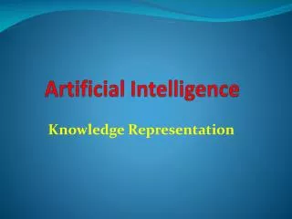
9. Table of Contents (Full Version)      Preface (html); chapter mapPart I Artificial Intelligence     1 Introduction      2 Intelligent Agents Part II Problem Solving     3 Solving Problems by Searching      4 Informed Search and Exploration      5 Constraint Satisfaction Problems     6 Adversarial Search Part III Knowledge and Reasoning     7 Logical Agents      8 First-Order Logic 9Inference in First-Order Logic10Knowledge RepresentationPart IV Planning 11 Planning (pdf) 12 Planning and Acting in the Real World Part V Uncertain Knowledge and Reasoning    13 Uncertainty14 Probabilistic Reasoning 15 Probabilistic Reasoning Over Time    16 Making Simple Decisions17 Making Complex Decisions Part VI Learning18 Learning from Observations19 Knowledge in Learning 20 Statistical Learning Methods 21 Reinforcement LearningPart VII Communicating, Perceiving, and Acting    22 Communication     23 Probabilistic Language Processing     24 Perception     25 Robotics Part VIII Conclusions    26 Philosophical Foundations   27 AI: Present and Future Topics Covered in CSE471

10. Representation Mechanisms: Logic (propositional; first order) Probabilistic logic Learning the models Search Blind, Informed SAT; Planning Inference Logical resolution Bayesian inference How the course topics stack up…

11. Pendulum Swings in AI • Top-down vs. Bottom-up • Ground vs. Lifted representation • The longer I live the farther down the Chomsky Hierarchy I seem to fall [Fernando Pereira] • Pure Inference and Pure Learning vs. Interleaved inference and learning • Knowledge Engineering vs. Model Learning vs. Data-driven Inference • Human-aware vs. Stand-Alone

12.  Class forum Class of 8/29

13. Agent Classification in Terms of State Representations

15. Markov Decision Processes Atomic Model for stochastic environments with generalized rewards • Based in part on slides by Alan Fern, Craig Boutilier and Daniel Weld • Some slides from Mausam/Kolobov Tutorial; and a couple from Terran Lane

16. Atomic Model for Deterministic Environments and Goals of Attainment Deterministic worlds + goals of attainment • Atomic model: Graph search • Propositional models: The PDDL planning that we discussed.. • What is missing? • Rewards are only at the end (and then you die). • What about “the Journey is the reward” philosophy? • Dynamics are assumed to be Deterministic • What about stochastic dynamics?

17. Atomic Model for stochastic environments with generalized rewards Stochastic worlds +generalized rewards An action can take you to any of a set of states with known probability You get rewards for visiting each state Objective is to increase your “cumulative” reward… What is the solution?

18. (Static vs. Dynamic) (Observable vs. Partially Observable) Environment (perfect vs. Imperfect) perception (Full vs. Partial satisfaction) (Instantaneous vs. Durative) action Goals (Deterministic vs. Stochastic) The $$$$$$ Question What action next?

19. Optimal Policies depend on horizon, rewards.. - - - -

20. 9/5/2012

21. Markov Decision Processes • An MDP has four components: S, A, R, T: • (finite) state set S (|S| = n) • (finite) action set A (|A| = m) • (Markov) transition function T(s,a,s’) = Pr(s’ | s,a) • Probability of going to state s’ after taking action a in state s • How many parameters does it take to represent? • bounded, real-valued (Markov) reward function R(s) • Immediate reward we get for being in state s • For example in a goal-based domain R(s) may equal 1 for goal states and 0 for all others • Can be generalized to include action costs: R(s,a) • Can be generalized to be a stochastic function • Can easily generalize to countable or continuous state and action spaces (but algorithms will be different)

22. Assumptions • First-Order Markovian dynamics (history independence) • Pr(St+1|At,St,At-1,St-1,..., S0) = Pr(St+1|At,St) • Next state only depends on current state and current action • First-Order Markovian reward process • Pr(Rt|At,St,At-1,St-1,..., S0) = Pr(Rt|At,St) • Reward only depends on current state and action • As described earlier we will assume reward is specified by a deterministic function R(s) • i.e. Pr(Rt=R(St) | At,St) = 1 • Stationary dynamics and reward • Pr(St+1|At,St) = Pr(Sk+1|Ak,Sk) for all t, k • The world dynamics do not depend on the absolute time • Full observability • Though we can’t predict exactly which state we will reach when we execute an action, once it is realized, we know what it is

23. Policies (“plans” for MDPs) • Nonstationary policy [Even though we have stationary dynamics and reward??] • π:S x T → A, where T is the non-negative integers • π(s,t) is action to do at state s with t stages-to-go • What if we want to keep acting indefinitely? • Stationary policy • π:S → A • π(s)is action to do at state s (regardless of time) • specifies a continuously reactive controller • These assume or have these properties: • full observability • history-independence • deterministic action choice If you are 20 and are not a liberal, you are heartless If you are 40 and not a conservative, you are mindless -Churchill Why not just consider sequences of actions? Why not just replan?

24. Value of a Policy • How good is a policy π? • How do we measure “accumulated” reward? • Value function V: S →ℝ associates value with each state (or each state and time for non-stationary π) • Vπ(s) denotes value of policy at state s • Depends on immediate reward, but also what you achieve subsequently by following π • An optimal policy is one that is no worse than any other policy at any state • The goal of MDP planning is to compute an optimal policy (method depends on how we define value)

25. Finite-Horizon Value Functions • We first consider maximizing total reward over a finite horizon • Assumes the agent has n time steps to live • To act optimally, should the agent use a stationary or non-stationary policy? • Put another way: • If you had only one week to live would you act the same way as if you had fifty years to live?

26. Finite Horizon Problems • Value (utility) depends on stage-to-go • hence so should policy: nonstationaryπ(s,k) • is k-stage-to-go value function for π • expected total reward after executing π for k time steps (for k=0?) • Here Rtand st are random variables denoting the reward received and state at stage t respectively

27. Computing Finite-Horizon Value • Can use dynamic programming to compute • Markov property is critical for this (a) (b) immediate reward expected future payoffwith k-1 stages to go π(s,k) 0.7 What is time complexity? 0.3 Vk Vk-1

28. ComputeExpectations Vt s1 ComputeMax s2 s3 s4 0.7 Vt (s1) + 0.3 Vt (s4) Vt+1(s) = R(s)+max { 0.4 Vt (s2) + 0.6 Vt(s3) } Bellman Backup How can we compute optimal Vt+1(s) given optimal Vt ? 0.7 a1 0.3 Vt+1(s) s 0.4 a2 0.6

29. Value Iteration: Finite Horizon Case • Markov property allows exploitation of DP principle for optimal policy construction • no need to enumerate |A|Tnpossible policies • Value Iteration Bellman backup Vk is optimal k-stage-to-go value function Π*(s,k) is optimal k-stage-to-go policy

30. V1 V3 V2 V0 s1 s2 0.7 0.7 0.7 0.4 0.4 0.4 s3 0.6 0.6 0.6 0.3 0.3 0.3 s4 V1(s4) = R(s4)+max { 0.7 V0 (s1) + 0.3 V0 (s4) 0.4 V0 (s2) + 0.6 V0(s3) } Optimal value depends on stages-to-go (independent in the infinite horizon case) Value Iteration

31. Value Iteration V1 V3 V2 V0 s1 s2 0.7 0.7 0.7 0.4 0.4 0.4 s3 0.6 0.6 0.6 0.3 0.3 0.3 s4 P*(s4,t) = max { }

32. 9/10/2012

33. Value Iteration • Note how DP is used • optimal soln to k-1 stage problem can be used without modification as part of optimal soln to k-stage problem • Because of finite horizon, policy nonstationary • What is the computational complexity? • T iterations • At each iteration, each of n states, computes expectation for |A| actions • Each expectation takes O(n) time • Total time complexity: O(T|A|n2) • Polynomial in number of states. Is this good?

34. Summary: Finite Horizon • Resulting policy is optimal • convince yourself of this • Note: optimal value function is unique, but optimal policy is not • Many policies can have same value

35. Discounted Infinite Horizon MDPs • Defining value as total reward is problematic with infinite horizons • many or all policies have infinite expected reward • some MDPs are ok (e.g., zero-cost absorbing states) • “Trick”: introduce discount factor 0 ≤ β < 1 • future rewards discounted by β per time step • Note: • Motivation: economic? failure prob? convenience?

36. Notes: Discounted Infinite Horizon • Optimal policy maximizes value at each state • Optimal policies guaranteed to exist (Howard60) • Can restrict attention to stationary policies • I.e. there is always an optimal stationary policy • Why change action at state s at new time t? • We define for some optimal π

37. Computing an Optimal Value Function • Bellman equation for optimal value function • Bellman proved this is always true • How can we compute the optimal value function? • The MAX operator makes the system non-linear, so the problem is more difficult than policy evaluation • Notice that the optimal value function is a fixed-point of the Bellman Backup operator B • B takes a value function as input and returns a new value function

38. Value Iteration • Can compute optimal policy using value iteration, just like finite-horizon problems (just include discount term) • Will converge to the optimal value function as k gets large. Why?

39. Convergence • B[V] is a contraction operator on value functions • For any V and V’ we have || B[V] – B[V’] || ≤ β || V – V’ || • Here ||V|| is the max-norm, which returns the maximum element of the vector • So applying a Bellman backup to any two value functions causes them to get closer together in the max-norm sense. • Convergence is assured • any V: ||V* - B[V] || = || B[V*] – B[V] || ≤ β||V* - V || • so applying Bellman backup to any value function brings us closer to V* by a factor β • thus, Bellman fixed point theorems ensure convergence in the limit • When to stop value iteration? when ||Vk -Vk-1||≤ ε • this ensures ||Vk –V*|| ≤ εβ /1-β

40. Contraction property proof sketch • Note that for any functions f and g • We can use this to show that • |B[V]-B[V’]| <= b|V – V’| f g

41. How to Act • Given a Vk from value iteration that closely approximates V*, what should we use as our policy? • Use greedy policy: • Note that the value of greedy policy may not be equal to Vk • Let VG be the value of the greedy policy? How close is VG to V*?

42. How to Act • Given a Vk from value iteration that closely approximates V*, what should we use as our policy? • Use greedy policy: • We can show that greedy is not too far from optimal if Vk is close to V* • In particular, if Vk is within ε of V*, then VG within 2εβ /1-β of V* (if ε is 0.001 and β is 0.9, we have 0.018) • Furthermore, there exists a finite εs.t. greedy policy is optimal • That is, even if value estimate is off, greedy policy is optimal once it is close enough

43. Improvements to Value Iteration • Initialize with a good approximate value function • Instead of R(s), consider something more like h(s) • Well defined only for SSPs • Asynchronous value iteration • Can use the already updated values of neighors to update the current node • Prioritized sweeping • Can decide the order in which to update states • As long as each state is updated infinitely often, it doesn’t matter if you don’t update them • What are good heuristics for Value iteration?

44. 9/14 (make-up for 9/12) • Policy Evaluation for Infinite Horizon MDPS • Policy Iteration • Why it works • How it compares to Value Iteration • Indefinite Horizon MDPs • The Stochastic Shortest Path MDPs • With initial state • Value Iteration works; policy iteration? • Reinforcement Learning start

45. Policy Evaluation • Value equation for fixed policy • Notice that this is stage-indepedent • How can we compute the value function for a policy? • we are given R and Pr • simple linear system with n variables (each variables is value of a state) and n constraints (one value equation for each state) • Use linear algebra (e.g. matrix inverse)

46. Policy Iteration • Given fixed policy, can compute its value exactly: • Policy iteration exploits this: iterates steps of policy evaluation and policy improvement 1. Choose a random policy π 2. Loop: (a) Evaluate Vπ (b) For each s in S, set (c) Replace π with π’ Until no improving action possible at any state Policy improvement

47. P.I. in action Iteration 0 Policy Value The PI in action slides from TerranLane’s Notes

48. P.I. in action Iteration 1 Policy Value

49. P.I. in action Iteration 2 Policy Value

50. P.I. in action Iteration 3 Policy Value