Understanding Inventory Management: Types, Systems, and Cost Implications
This document provides an overview of inventory management, outlining its key purposes such as meeting expected demand, absorbing fluctuations, and protecting against price increases. It covers different types of inventory including raw materials, work-in-process, and finished goods, as well as the classification of inventory items. Additionally, it explains inventory systems such as perpetual and periodic review, performance measures, and costs associated with inventory methods like the EOQ model. A practical example of the EOQ model is presented, illustrating its application in managing inventory effectively.

Understanding Inventory Management: Types, Systems, and Cost Implications
E N D
Presentation Transcript
Inventory Management COB 300 C Busing
Purposes of Inventory • Meet expected demand • Absorb demand fluctuations • Protect against unexpected increases in demand • Decouple stages in the production process • Take advantage of quantity discounts • Hedge against possible price increases • Protect against disruption in delivery from suppliers
Types of Inventory • Raw materials • Work-in-process (WIP) • Finished goods • Replacement parts • Supplies • Transportation
Dependent andIndependent Demand • Dependent Demand = usually generated by a company’s own production process • Independent Demand = usually from outside sources such as customers
Types of Inventory Systems • Perpetual (Continuous Review) • Inventory level continuously monitored • Transactions recorded as they occur • Maintain specific level of inventory • Periodic • Inventory counted only at regular intervals • Inventory depends upon demand
ABC Classification of Inventory Items Cumulative Annual Unit Annual Dollar % Annual % Annual Item Demand Cost Usage Dollar Usage Dollar Usage Classification 1 2 3 4 5 6 7 8 9 10 48.91 78.25 84.77 89.99 93.25 95.21 96.90 98.53 99.67 100.00 A A B B B C C C C C $ 150,000 90,000 20,000 16,000 10,000 6,000 5,200 5,000 3,500 1,000 306,700 48.91 29.34 6.52 5.22 3.26 1.96 1.69 1.63 1.14 .33 $ 30 450 10 20 10 5 4 2 1 20 5,000 200 2,000 800 1,000 1,200 1,300 2,500 3,500 500
Aggregate Performance Measures -Average inventory investment -Turnover ratio - Days of inventory Annual cost of goods sold Average inventory investment Days per year Turnover ratio
Inventory Ordering Costs Fixed Staffing Office and equipment Variable Shipping Order placing Setup cost Lost materials Receiving and inspection Inventory Holding Costs Fixed Warehouse-capital Property taxes Warehouse-operating Personnel Variable Cost of capital Insurance Losses Inventory taxes Rental costs Costs of Inventory
EOQ Model Assumptions 1. Constant known demand rate 2. Cost per unit fixed 3. Instantaneous replenishment 4. Ordering and carrying cost known and independent
EOQ Model D = Annual Demand rate Co = Variable ordering cost Ch = Variable holding cost
EOQ Model D = Annual Demand rate Co = Variable ordering cost Ch = Variable holding cost D = 1,000 units/year Co = $50 per order Ch = $5 per unit per year
Total Annual Variable Cost (Slide 1 of 2) D Annual variable ordering cost = Co Annual variable holding cost = Ch Total annual variable cost = Ch + Co Q Q 2 Q D 2 Q
Total Annual Variable Cost (Slide 2 of 2) D = 1,000 Co= $50 Ch = $5 EOQ = 141.42 Total annual variable costs 141.42 1,000 2 141.42 140 1,000 2 140 145 1,000 2 145 200 1,000 2 200 EOQ: (5) + (50) = $707.11 (5) + (50) = $707.14 140: (5) 145: + (50) = $707.33 (50) = $750.00 200: (5) +
Quantity Produced During Replenishment Period vs. Maximum Inventory
Finite Replenishment Rate Model D = annual demand rate Co = Variable ordering cost Ch = variable holding cost d = dally demand rate p = daily production rate Total annual variable costs D = 1,000; Co = $50; Ch = $5; d = 4; p = 10
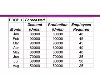
Homework • Problem 1 (Handout); 3,4,8 (ch. 9)