Unit 1 Overview

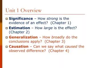
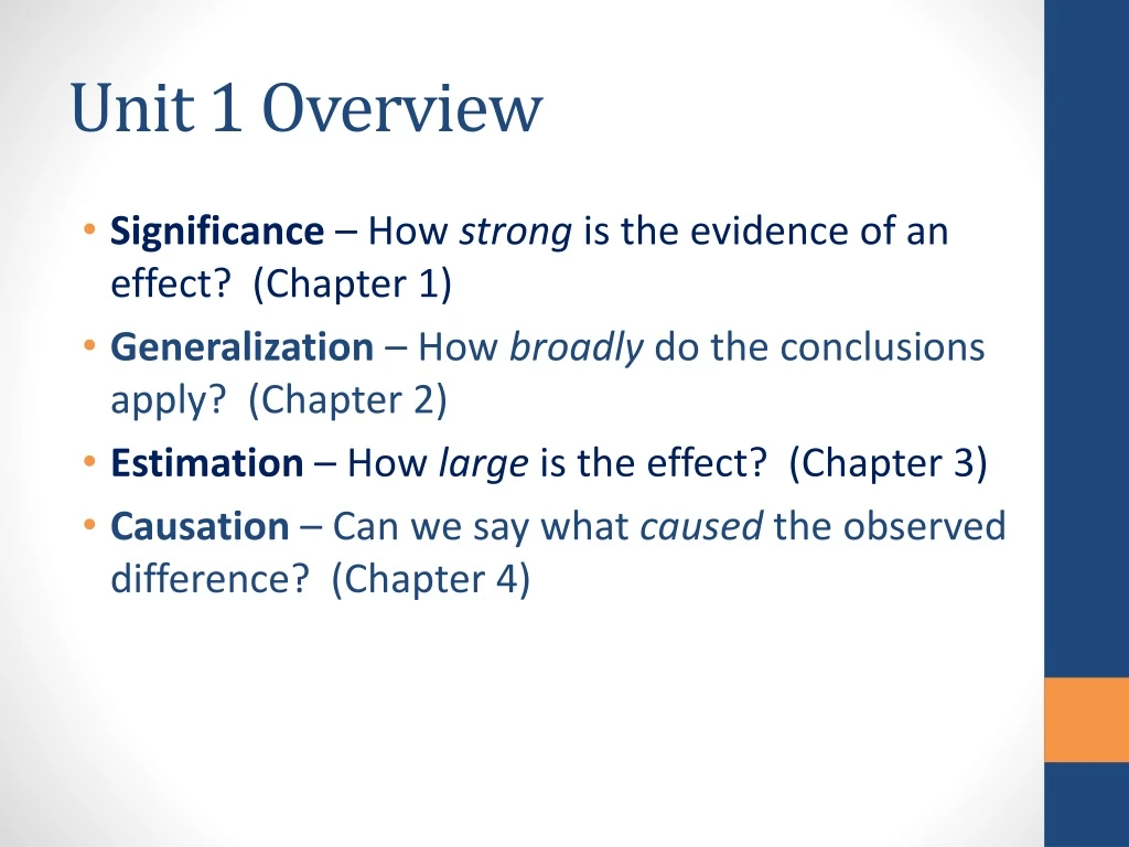
1. Unit 1 Overview • Significance – How strong is the evidence of an effect? (Chapter 1) • Generalization – How broadly do the conclusions apply? (Chapter 2)  • Estimation – How large is the effect? (Chapter 3) • Causation – Can we say what caused the observed difference? (Chapter 4)

2. Terminology from Preliminaries • The individual entities on which data are recorded are called observational units. • The recorded characteristics of the observational units are the variablesof interest. • Variables can be: • Quantitative • You can add, subtract, etc. with the values. • Height, weight, distance, time… • Categorical • Labels for which arithmetic does not make sense. • Sex, ethnicity, eye color…

3. Chapter 1Significance: How Strong is the Evidence?

4. Section 1.1: Introduction to Chance Models

5. Example 1.1: Dolphin Communication

6. U.S. Navy Marine Mammal Program The dolphin communication study that we will be looking at was done under a contract with the navy in the 1960s. The navy still has a marine mammal program. Dolphins and sea Lions Ship and harbor protection Mine detection Equipment recovery

7. Other Military Animals

8. Can dolphins communicate abstract ideas? Buzz Doris

9. Step 1: Learn the Signals

10. Step 1: Learn the Signals

11. Step 2: Learn the Order Buzz Doris

12. Step 3: Communicate! LEFT ! Buzz Doris

13. The statistic • In one set of trials, Buzz chose the correct button 15 out of 16 times. • So our sample proportion is 15/16 = 0.9375. • Based on the results, do you think Buzz knew which button to push or is he guessing? • What sort of results would lead you to think he is just guessing? He is understanding?

14. Possible Explanations • There are two possible reasons why Buzz chose the correct button so many times. • He is just randomly guessing and got 15 out of 16 correct just by chance. • He was doing something other than just guessing and was understanding what Doris was telling him. • We want to model the random guessing and see how Buzz’s result fits in this model. • How might we model the situation where Buzz is just guessing (our chance model)?

15. Simulation vs. Real Study

16. Modeling Doris and Buzz • Flip Coins • One Proportion Applet

17. Three S Strategy • Statistic: Compute the statistic from the observed data. • Simulate: Identify a model that represents a chance explanation. Repeatedly simulate values of the statistic that could have happened when the chance model is true and form a distribution. • Strength of evidence: Consider whether the value of the observed statistic is unlikely to occur when the chance model is true.

18. Terminology • What are the observational units in the Buzz and Doris Experiment? How many are there? • What is the variable? Is it categorical or quantitative? • The statistic (lower case s) is the proportion of times Buzz pushed the correct button. (15/16) • The parameter is Buzz’s probability (long-term proportion) of choosing the correct button.

19. Statistic & Parameter • A statistic is a known quantity---like 15/16 • A parameter, while some fixed number, is not generally known. • A statistic is measured on a sample. • A parameter is measured on a process (and as we will see in the next chapter, a population) • We ask questions about the parameter (like does Buzz choose correctly 50% of the time in the long run) and then answer these questions based on the chance that the statistic would occur if the parameter was a certain value (like 50%).

20. Doris and Buzz Redo • Instead of a canvas curtain, Dr. Bastian constructed a wooden barrier between Buzz and Doris. • When tested, Buzz pushed the correct button only 16 out of 28 times. • Are these results statistically significant? • Let’s go to the applet to check this out.

21. Doris and Buzz Video

23. Learning Objectives for Section 1.1 • Be able to describe how to use coin tossing to simulate outcomes from a chance model of the random choice between two events. • Be able to use the One Proportion applet to carry out the coin tossing simulation. • Implement the 3S strategy: find a statistic, simulate results from a chance model, and comment on strength of evidence against observed study results happening by chance alone.

24. Learning Objectives for Section 1.1 • Recognize the difference between parameters and statistics. • Identify whether or not study results are statistically significant or if the chance model is a plausible explanation for the data. • Be able to differentiate between saying the chance model is plausible and the chance model the correct explanation for the observed data. 

25. Exploration 1.1: Can Dogs Understand Human Cues? (pg. 30) • Dogs were positioned 2.5 m from experimenter. • On each side of the experimenter were two cups. • The experimenter would perform some human cue (pointing, bowing or looking) towards one of the cups. (Non-human cues were also done.) • We will look at Harley’s results.

26. Section 1.2: Measuring Strength of Evidence • In the previous section we preformed tests of significance. • In this section we will make things slightly more complicated, formalize the process, and define new terminology.

27. We could take a look at Rock-Paper-Scissors-Lizard-Spock • Scissors cut paper • Paper covers rock • Rock crushes lizard • Lizard poisons Spock • Spock smashes scissors • Scissors decapitate lizard • Lizard eats paper • Paper disproves Spock • Spock vaporizes rock • (and as it always has) Rock crushes scissors

28. Rock-Paper-Scissors • Rock smashes scissors • Paper covers rock • Scissors cut paper • Are these choices used in equal proportions (1/3 each)? • One study suggests that scissors are chosen less than 1/3 of the time.

29. Rock-Paper-Scissors • Suppose we are going to test this with 12 players each playing once against a computer. • What are the observational units? • What is the variable? • Even though there are three outcomes, we are focusing on whether the player chooses scissors or not. This is called a binary variable since we are focusing on 2 outcomes (not both necessarily equally likely).

30. Terminology: Hypotheses • When conducting a test of significance, one of the first things we do is give the null and alternative hypotheses. • The null hypothesis is the chance explanation. • Typically the alternative hypothesis is what the researchers think is true.

31. Hypotheses from Buzz and Doris • Null Hypothesis: Buzz will randomly pick a button. (He chooses the correct button 50% of the time, in the long run.) • Alternative Hypothesis: Buzz understands what Doris is communicating to him. (He chooses the correct button more than 50% of the time, in the long run.) These hypotheses represent the parameter (long run behavior) not the statistic (the observed results).

32. Hypotheses for R-P-S in words • Null Hypothesis: People playing Rock-Paper-Scissors will equally choose between the three options. (In particular, they will choose scissors one-third of the time, in the long run.) • Alternative Hypothesis: People playing Rock-Paper-Scissors will choose scissors less than one-third of the time, in the long run. Note the differences (and similarities) between these hypotheses and those for Buzz and Doris.

33. Hypotheses for R-P-S using symbols • H0: π = 1/3 • Ha: π < 1/3 where π is players’ true probability of throwing scissors

34. Setting up a Chance Model • Because the Buzz and Doris example had a 50% chance outcome, we could use a coin to model the outcome from one trial. What could we do in the case of Rock-Paper-Scissors?

35. Three S Strategy • Statistic: Compute the statistic from the observed data. [In a class of 12 students, 2 picked scissors. This sample proportion can be described using the symbol (p-hat)]. • Simulate: Identify a model that represents a chance explanation. Repeatedly simulate values of the statistic that could have happened when the chance model is true and form a distribution. • Strength of evidence: Consider whether the value of the observed statistic is unlikely to occur when the chance model is true.

36. Applet • We will use the One Proportion Applet for our test. • This is the same applet we used last time except now we will change the proportion under the null hypothesis. • Let’s go to the applet and run the test. (Notice the use of symbols in the applet.)

37. Null Distribution

38. P-value • The p-value is the proportion of the simulated statistics in the null distribution that are at least as extreme (in the direction of the alternative hypothesis) as the value of the statistic actually observed in the research study. • We should have seen something similar to this in the applet: • Proportion of samples: 173/1000 = 0.173

39. What can we conclude? • Do we have strong evidence that less than 1/3 of the time scissors gets thrown? • How small of a p-value would you say gives strong evidence? • Remember the smaller the p-value, the stronger the evidence against the null.

40. Guidelines for evaluating strength of evidence from p-values • p-value >0.10, not much evidence against null hypothesis • 0.05 < p-value < 0.10, moderate evidence against the null hypothesis • 0.01 < p-value < 0.05, strong evidence against the null hypothesis • p-value < 0.01, very strong evidence against the null hypothesis

41. What can we conclude? • So we do not have strong evidence that fewer than 1/3 of the time scissors is thrown. • Does this mean we can conclude that 1/3 of the time scissors is thrown? • Is it plausible that 1/3 of the time scissors is thrown? • Are other values plausible? Which ones? • Suppose 1/12 of our sample chose scissors instead of 2/12. How would the p-value change? • What could we do in our study design to have a better chance of getting strong evidence for our alternative hypothesis?

42. Summary • The null hypothesis (H0) is the chance explanation. (=) • The alternative hypothesis (Ha) is you are trying to show is true. (< or >) • A null distribution is the distribution of simulated statistics that represent the chance outcome. • The p-value is the proportion of the simulated statistics in the null distribution that are at least as extreme as the value of the observed statistic.

43. Summary • The smaller the p-value, the stronger the evidence against the null. • P-values less than 0.05 provide strong evidence against the null. • πrepresents the population parameter • represents the sample proportion • n represents the sample size

44. Learning Objectives for Section 1.2 • Use appropriate symbols for parameter and statistic. • State the null and the alternative hypotheses in words and in terms of the symbol π, the probability. • Explain how to conduct a simulation using a null hypothesis probability that is not 50-50. • Use the One Proportion applet to obtain the p-value after carrying out an appropriate simulation.

45. Learning Objectives for Section 1.2 • Explain what a p-value means. • Explain why a smaller p-value provides stronger evidence against the null hypothesis. • State a conclusion about the alternative hypothesis and null hypothesis based on the p-value. • Anticipate the location of the center of the null distribution and how it changes based on whether you are using proportion or count as the statistic. 

46. Exploration 1.2: Tasting Water (pg. 41) • Can people tell the difference between bottled and tap water? • Researchers had their subjects taste 4 glasses of water, 3 filled with bottled water and 1 filled with tap water. They asked which water they preferred.

47. Alternative Measure of Strength of Evidence Section 1.3

48. Criminal Justice System vs. Significance Tests • Innocent until proven guilty. We assume a defendant is innocent and the prosecution has to collect evidence to try to prove the defendant is guilty. • Likewise, we assume our chance model (or null hypothesis) is true and we collect data and calculate a sample proportion. We then show how unlikely our proportion is if the chance model is true.

49. Criminal Justice System vs. Significance Tests • If the prosecution shows lots of evidence that goes against this assumption of innocence (DNA, witnesses, motive, contradictory story, etc.) then the jury might conclude that the innocence assumption is wrong. • If after we collect data and find that the likelihood (p-value) of such a proportion is so small that it would rarely occur by chance if the null hypothesis is true, then we conclude our chance model is wrong.

50. Review • In the water tasting exploration, you could have obtained a null distribution similar to the one shown here. (H0: π = 0.25, Ha: π < 0.25 and = 3/27 = 0.1111) • What does a single dot represent? • What does the whole distribution represent? • What is the p-value for this simulation? • What does this p-value mean?