Download

1 / 46
470 likes | 707 Vues
Description of measurement data. Prof. Yi-xiong Lei (1021305). Distribution of frequency To summarize the data or describe the distri- bution of frequency, frequency table or graph is the common way. The type of distribution: Normal distribution Skewness distribution

E N D
Description of measurement data Prof. Yi-xiong Lei (1021305)
Distribution of frequency • To summarize the data or describe the distri- • bution of frequency, frequency table or graph • is the common way. The type of distribution: • Normal distribution • Skewness distribution • Positive skewness distribution • Negative skewness distribution
If we are faced with a large amount of data, we want to describe its more important features more concisely. Usually we describe the data from two aspects. Measures of Location Central tendency (central position) Measures of Spread Tendency of dispersion (variation)
* Normal distribution Table2-1. Frequency Distribution of Red Blood Cells (1012/L) among 130 Normal Male Adults in Some District RBCsMarkFrequency 3.70~ | | 2 3.90~ | | | | 4 4.10~ 正 | | | | 9 4.30~ 正正正 | 16 4.50~ 正正正正 | | 22 4.70~ 正正正正正 25 4.90~ 正正正正 | 21 5.10~ 正正正 | | 17 5.30~ 正 | | | | 9 5.50~ | | | | 4 5.70~5.90 | 1 Total —— 130
﹡ Positive skewness distribution Table 2-2. Frequency Distribution of Hair Hg Value (μg/g) among 238 Normal Adults Value of hair HgFrequency Accumulative FrequencyAF (%) (1) (2) (3) (4)=(3)/238 0.3~ 20 20 8.4 0.7~ 66 86 36.1 1.1~ 60 146 61.3 1.5~ 48 194 81.5 1.9~ 18 212 89.1 2.3~ 16 228 95.8 2.7~ 6 234 98.3 3.1~ 1 235 98.7 3.5~ 0 235 98.7 3.9~ 3 238 100.0
﹡ Negative skewness distribution Table 2-3. Frequency Distribution of Patients who die of Malignant Tumors in some year and district Age (yr.)No. of DeathAccumulative FrequencyAF (%) 0~ 5 5 0.42 10~ 12 17 1.41 20~ 15 32 2.66 30~ 76 108 8.98 40~ 189 297 24.69 50~ 234 531 44.14 60~ 386 917 76.23 70~ 286 1203 100.00
Figure 2-1. Frequency Distribution of Serum Cholesterol (mg/dl) among 200 Normal Adults in Some District
2. Average What measure is used to describe the central tendency? It is the average including mean, geometric mean and median. Mean,symbolized by, -bar AverageGeometric mean, symbolized by G Median, symbolized by M
1). Mean,is suitable to the data distri-buted in normal distribution or at least symmetric distribution. • x1+ x2+……+ xn ∑ x • Formula(1) x = = n n • f 1x1 + f 2x2 + ……+f kxk ∑ fx • Formula(2) x = = • f 1 +f 2+……+f k n The formula (1) is for original data (direct method) The formula (2) is for frequency table (weighing method)
RBCsMiddle value (X)Frequency (f) f X 3.80~ 3.90 2 7.8 4.00~ 4.10 6 24.6 4.20~ 4.30 11 47.3 4.40~ 4.50 25 112.5 4.60~ 4.70 32 150.4 4.80~ 4.90 27 132.3 5.00~ 5.10 17 86.7 5.20~ 5.30 13 68.9 5.40~ 5.50 4 22.0 5.60~ 5.70 2 11.4 5.80~6.00 5.90 1 5.9 Total — 140(∑f) 669.8 (∑f x) 669.8 140 • ∑f x • ∑f X= =4.78 (×1012/L) = Table2-4. Frequency Distribution of Red Blood Cells (1012/L) among 140 Normal Male Adults in Some District
(1) G = n √ x1 · x2 … xn lgx1+lgx2+…+lgxn∑ lgx G = lg–1 = lg–1 n n f1lgx1+f2lgx2+…+fklgxk∑f lgx (2) G = lg–1 = lg–1 ∑f ∑f 2). Geometric mean, issuitable to the data distributed in positive skewed distribution or logarithm normal distribution. The formula (1) is for original data (direct method) The formula (2) is for frequency table (weighing method)
lgx1+lgx2+…+lgxn 〔 〕 G = lg –1 ∑ lgx = lg–1 1+2+3+4+5 5 n = lg –1 〔 〕 = lg –1 3 n 10+100+… … … +100000 5 = ∑x n X= There are 6 items of serum antibodies, the concentrations respectively are 1:10, 1:100, 1:1000, 1:10000 and 1:100000, what is the average concentration ? Wrong =22222 =1000 Right 1:1000
G = 109.79 52 ∑f lgx 〔 〕 = Lg –1 〔 〕 Lg –1 ∑f Table 2-5. The special serum antibodies’ concentrations after one month when 52 susceptible children immunized with measles vaccine Ab concent.Children (f) Reciprocal (x) lgx flgx 1: 40 3 40 1.602 4.81 1: 80 22 80 1.903 41.87 1: 160 17 160 2.204 37.47 1: 320 9 320 2.505 22.55 1: 640 0 640 2.806 0.00 1:1280 1 1280 3.107 3.11 Total ∑52 — — 109.79 =129.2 average antibodies’ concentration 1:129
M = X n+1 (n is odd No.) 2 1 or M= X n + X n (n is even No.) 2 2 2 +1 3).Median, is suitable to all kinds of data but it is poor attribution for further ana-lysis comparing to mean. The following formula is for original data (direct method):
For example : There are 9cases, the latent period is 2,3,3,3,4,5,6,9,16 days, please calculate their average latent period. M = X(n+1)/2 = X(9+1)/2 = X5 = 4 (days)
4).Median and percentile for the data from a frequency table we do not know the exactly value of median, using the following formula for median or percentile Px=L+i / fx(n.x% - ΣfL) (frequency table method or percentile method)
Px=L+i / fx(n.x% - ΣfL) X : percentile; L : the low limit of group where percentile located in i : the interval; f : frequency in the group; n : the total cases; ΣfL : accumulative frequency that less than L. If Px = 50% = M, using following formula: M=L+i/f(n/2-ΣfL)
Table 2-6. The calculations of median and percentile of latent period of food poisoning among 164 cases Latent period (hours) Cases ( f ) Accumulative frequency(Σf) Accumulative frequency(%) 0~ 25 25 15.2 12~ 58 83 50.6 24~ 40 123 75.0 36~ 23 146 89.0 48~ 12 158 96.3 60~ 5 163 99.4 72~84 1 164 100.0
Median calculation: from table 2-6, accumulative frequency 50% is within the group “12~”,L=12,i=12, f=58, ΣfL=25, n=164 M=L+i/f(n/2-ΣfL)=12+12/58(164/2-25)=23.8 (hrs) Percentile (Px) calculation: when P95, x=95,accumulative frequency 95% is within the group “48~”,L=48,i=12,fx=12, ΣfL=146, n=164 P95=48+12/12(164×95%-146)=57.8 (hrs)
Measures of Spread Tendency of dispersion (variation) Prof. Yi-xiong Lei (1021305)
3. Measures of Spread There are some features to describe the distri -bution of different data. Two common features we might be interested in are: > What is the typical (average) value of a variable (what is its location)? > How much variability is there in the data (how much does it spread out)?
The common variations are the following: Range, symbolized by R Interval of quartile, symbolized by Q Variations Variance, symbolized by2, S2 Standard deviation, symbolized by, S Coefficient of variation, symbolized by CV
1) Range,is suitable to all kinds of data but it is a poor measure of variability because it is based on only two extreme observations. R = Xmax - Xmin
2) Interval of quartile (Q), is the scale of variation, from the 25 percentile(P25)to the 75 percentile(P75). Quartile is suitable to all kinds of data, especially for the data of skewness distribution, it’s application is better than range. Using the following formula to calculate the quartile (Q) Px=L+i / fx(n.x% - ΣfL) The example above is Q = Qu-QL= P75 - P25 = 36.0 -15.3=20.7(hrs)
3) Variance(2, s2)and Standard deviation(SD or S) They are the important variability measures and suitable to data of normal distribution ∑( X— μ) 2 ∑(X— μ) 2 σ2 = σ= N N ∑( X— X) 2 ∑( X— X) 2 S2 = S = n — 1 n — 1
The Formula for standard deviation ∑X2 — ( ∑X ) 2 / n Direct S = method√ n — 1 ∑f X2 — ( ∑ f X) 2 / n Weighing S = method√ n — 1
∑X = 813 ∑X2 = 133317 √ 133317 – (813)2/ 5 = 5 –1 = 19.49 mmHg √ S = ∑X2 - ( ∑X ) 2 / n n - 1 For example, 5 persons’ diastolic blood pressure are: 162, 145, 178, 142, 186 (mmHg)
√ √ 3224.20 – (669.8)2/n = S = ∑fX2 - ( ∑fX ) 2 / n 140 - 1 n - 1 Table2-7. Frequency Distribution of Red Blood Cells (1012/L) among 140 Normal Male Adults in Some District RBCsMiddle value (X)Frequency (f) f Xf X 2 3.80~ 3.90 2 7.8 30.42 4.00~ 4.10 6 24.6 100.86 4.20~ 4.30 11 47.3 203.39 4.40~ 4.50 25 112.5 506.25 4.60~ 4.70 32 150.4 706.88 4.80~ 4.90 27 132.3 648.27 5.00~ 5.10 17 86.7 442.17 5.20~ 5.30 13 68.9 365.17 5.40~ 5.50 4 22.0 121.00 5.60~ 5.70 2 11.4 64.98 5.80~6.00 5.90 1 5.9 5.90 Total(∑) — 140 669.83224.20 =0.38
4)Coefficient of variation (CV),is that the standard deviation divided by mean and then it is comparable between different data. If comparing the variability among two or more than two groups that their metric units are different or their means are obvious different values you may calculate their CV CV = s / x × 100%
For example:Someone randomly measure the heights (cm) and weighs (kg) of 110 health male students in the age of 20 at a city in 2004, please compare the variability between heights (cm) and weighs (kg) For heights, knowing: = 172.73 (cm), S =4.09 (cm) For weights, knowing: = 55.04 (kg), S =4.10 (kg) For heights, CV = 4.09 / 172.73 ×100% = 2.37% For weights, CV = 4.10 / 55.04 ×100% = 7.45% Indicating the index of heights is more stable.
5) Applications of standard deviation (A) Showing the variability (spread) of observations; (B) Describing the features of normal distribution of data when combined with mean; (C) Estimating the medical reference range when combined with mean; (D)Calculating the standard error of mean when combined with sample size (n).
Normal Distribution & It’s application Prof. Yi-xiong Lei (1021305)
Normal distribution curve Frequency (f ) f 125 129 133 137 141 145 149 153 157 161 Heights (cm) Figure 2-1. Frequency distribution and its curve of heights among 120 health boys at the age of 12 4. Normal Distribution and Application (1) What means the normal distribution
f(X) F(X) -∞ +∞ The normal distribution is defined by the function: f(X)
(2) The attributes of normal distribution A. The shape of curve likes a bell and it is symmetric. B. The top of peak locates in center (mean, median) . C. There are two parameter and , marking N (, ) . D. There is a rule to estimate the area of distribution, the area within the curve is 1 or 100% . Parameter Parameter
(3) The area rule of normal distribution μ±1σ the area rule is 68.27% μ±1.96σ the area rule is 95.00% μ±2.58σ the area rule is 99.00% If n>100,μreplace by x,σreplace by s - Normal distribution curve 2.5% 0.5% -2.58 -1.96 -1 +1 +1.96 +2.58
(4) Standard normal distribution Ifμ=0, σ=1, Nd Snd If u=(X-μ)/σ, u observed a snd N(0,1) So, standard normal distribution means u-distribution (u) (u) -∞ 0 U +∞
(5) The area rule of Snd -1< u < +1, the area rule is 68.27% -1.96 < u < +1.96, the area rule is 95.0% -2.58 < u < +2.58, the area rule is 99.0% Standard normal distribution -2.58 -1.96 -1 0 +1 +1.96 +2.58
(6) Application of normal distribution (A) Estimating frequency distribution 130 newborn’s weight: X-bar=3200g, s=350g Please estimate the ratio of the low weight. (The standard of low weight: X=2500g) u=(x-µ)/ = (2500-3200)/350= -2 See table 2-11 in the book (p39): (-2)= 0.0228= 2.28% (the ratio of the low weight) 130 2.28% = 2.96 = 3 (person No. of of the low weight)
(B)The estimation of a reference range: Reference range, meaning “normal range”, is the value range of most normal individuals. (The most means 80%, 90%, 95% or 99%) Normal False negative Patient False positive Upper limit (95%)
For example Red blood cells (RBC): 3.5~5.0 (×1012/L) White blood cells (WBC): 4~10 (×109/L) Cholesterol in blood: 3.1~5.7 mmol /L Lead in urine: < 0.08 mg /L • Two methods to estimate a reference range: • Method of normal distribution • Method of percentiles
If the frequency distribution is close to the normal distribution, we may estimate the reference range according to the method of normal distribution or percentiles. x ± us (two side 1- range) x + us or x - us (one side 1- range) Table 2-8. Common u- value Reference range Two side One side 80 % 1.282 0.842 90 % 1.645 1.282 95 % 1.960 1.645 99 % 2.576 2.326
For example:Someone randomly measure the heights (cm) of 110 health male students in the age of 20 at a city in 2004. For heights, =172.73 (cm), S=4.09 (cm), please calculate the reference range of the height. Calculating two side 95% reference range: x ± us x ±1.96·s x ±1.96s = 172.73 ± 1.96 × 4.09 95% reference range of the students’ heights is 164.71~180.75 (cm)
If the frequency distribution is skewed, we may estimate the reference range by percentiles. 95% two side reference range: P2.5 ~ P97.5 95% one side range in upper limit: < P95 95% one side range in lower limit: > P5 (C)The control of data quality χ± 3s