PATTERNS IN THE KPZ EQUATION
PATTERNS IN THE KPZ EQUATION. Mapping of stochastic equations to Hamilton equations of motion. Hans Fogedby Aarhus University and Niels Bohr Institute Denmark. Outline. Equilibrium Non equilibrium Quantum analogue Weak noise - WKB Dynamical equations of motion Phase space discussion

PATTERNS IN THE KPZ EQUATION
E N D
Presentation Transcript
PATTERNS IN THE KPZ EQUATION Mapping of stochastic equations to Hamilton equations of motion Hans Fogedby Aarhus University and Niels Bohr Institute Denmark
Outline • Equilibrium • Non equilibrium • Quantum analogue • Weak noise - WKB • Dynamical equations of motion • Phase space discussion • Brownian motion • Oscillator • Finite-time-singularity • Kardar-Parisi-Zhang equation for interface • Summary and conclusion NON EQUILIBRIUM
EQUILIBRIUM Ensemble known - Boltzmann/Gibbs scheme • P0: Distribution • H(C): Hamiltonian • C: Configuration • kBT: Temperature • F: Free energy • S: Entropy Boltzmann factor Partition function Thermodynamics Example: • HI: Ising Hamiltonian • σi : Spin, σi =±1 • J: NN Coupling • {σi}: Configuration • H: Magnetic field • M: Magnetic moment Ising model NON EQUILIBRIUM
Open systems Biophysics Soft matter Turbulence Interface growth etc NON EQUILIBRIUM Ensemble unknown - Master/Langevin/Fokker-Planck scheme Master equation Langevin equation Fokker-Planck equation NON EQUILIBRIUM
Distribution corresponds to wave function Fokker-Planck equation corresponds to Schrödinger equation Noise yields kinetic energy Drift yields potential energy Small noise strength corresponds to small Planck constant Weak noise corresponds to small quantum fluctuations i.e. the correspondence limit QUANTUM ANALOGUE Fokker Planck equation Diffusion Drift Transformation Schrödinger equation Kinetic energy p-dependent potential NON EQUILIBRIUM
WEAK NOISE Langevin equation • Noise drives x into a stationary • stochastic state • Noise strength singular parameter • Δ=0, relaxational behavior • Δ~0, stationary behavior • Cross over time diverges as Δ → 0 Drift Noise Noise correlations Noise strength Working hypothesis: Weak noise limit captures interesting physics NON EQUILIBRIUM
WEAK NOISE - WKB Fokker-Planck equation Action WKB ansatz Variational principle Hamilton-Jacobi equation • Principle of least action operational • in weak noise limit • Stochastic problem replaced by • dynamical problem • Application of dynamical system theory • Dynamical action S is weight function Hamiltonian NON EQUILIBRIUM
Solve equations of motion for orbit from xi to x in time T Momentum p is ”slaved” variable Evaluate action S for orbit Evaluate transition probability according to WKB ansatz Stationary distribution obtained in long time limit for fixed x DYNAMICAL EQUATIONS Hamiltonian Langevin equation Equations of motion Weak noise recipe Noise replaced by momentum Equation for momentum Action and distribution WKB NON EQUILIBRIUM
PHASE SPACE DISCUSSION Hamiltonian Equations of motion Action • Long time orbits on H=0 manifolds • H=0 manifolds yield stationary state • Saddle point - infinite waiting time • (Markov behavior) NON EQUILIBRIUM
Basic random process Model for diffusion Wide applications in statistical physics BROWNIAN MOTION Solutions Action and distribution Langevin equation Gaussian, width ~T Phase space Hamiltonian (free particle) Equations of motion NON EQUILIBRIUM
OSCILLATOR (overdamped) • Simple random process • Wide applications in statistical physics and biophysics • E.g. suspended Brownian particle in viscous medium Mean square displacement Fokker-Planck equation Distribution Langevin equation Stationary distribution Gaussian NON EQUILIBRIUM
Weak noise approach Langevin equation Action Hamiltonian Distribution Stationary distribution Equations of motion Gaussian NON EQUILIBRIUM
Phase space discussion Stationary manifold Finite time orbit Infinite time orbit Transient manifold Saddle point (long time orbit passes close to SP) NON EQUILIBRIUM
FINITE-TIME-SINGULARITIES Generic model with singularity FTS encountered in … • Stellar structure • Turbulent flow • Bacterial growth • Euler flow • Free surface flow • Econophysics • Geophysics • Material physics Finite-time solution Sharp event horizon NON EQUILIBRIUM
NOISY FINITE-TIME-SINGULARITY Absorbing state distribution W(t) • Noise smears out singularity • Event horizon becomes fuzzy • e.g. hydrodynamical flow on nano scale near finite-time singularity Generic model with noise Noise intrinsic or thermal, Δ ≈ T Power law behavior Scaling exponent NON EQUILIBRIUM
Weak noise approach FTS model with noise Phase space Hamiltonian Equations of motion Long time analysis yields absorbing state distribution and scaling exponent Action and distribution NON EQUILIBRIUM
KARDAR PARISI ZHANG EQUATION • Generic non equilibrium model • Describes aspects of growing interface • Field theoretical Langevin equation • Scaling properties • Related to turbulence • Related to disordered systems • Weak noise method can be applied NON EQUILIBRIUM
KARDAR PARISI ZHANG EQUATION • h(r,t): height profile • ν: damping • λ: growth parameter • F: drift • η(r,t): noise • Δ: noise strength NON EQUILIBRIUM
KPZ - scaling Dynamical scaling hypothesis • Saturation width: w • System size: L • Roughness exponent: ς • Dynamic exponent: z • Scaling function: F NON EQUILIBRIUM
KPZ - scaling DRG phase diagram • Dynamical Renormalization • Group (DRG) calculation • d=2 lower critical dimension • Expansion in d-2 • Strong coupling fixed point • in d=1, z=3/2 • Kinetic phase transition for • d>2 • d=4 upper critical dimension Scaling law DRG equation NON EQUILIBRIUM
Weak noise approach KPZ equation Action Cole-Hopf transformation to diffusive field w Distribution Hamiltonian Phase space Field equations of motion NON EQUILIBRIUM
Pattern formation Program • Find localized solutions to static field equations • Boost static solutions to moving growth modes • Construct dynamical network of dynamical growth modes New parameters Diffusion equation Static field equations Non linear Schrödinger equation NON EQUILIBRIUM
Diffusion equation Radial diffusion equation Solutions for w, height h and slope u NON EQUILIBRIUM
Non linear Schrödinger equation Radial NLSE Solutions for w, height h and slope u NON EQUILIBRIUM
Galilei transformation Galilei boost Growth modes in 2D Moving growth modes NON EQUILIBRIUM
Dynamical network NON EQUILIBRIUM
Growth in d=1 NON EQUILIBRIUM
Dipole modes in 2D Moving slope mode Moving height mode NON EQUILIBRIUM
4-monopole height profile in 2D NON EQUILIBRIUM
SUMMARY AND CONCLUSION • Nonperturbative asymptotic weak noise approach • Equivalent to the WKB approximation in QM • Stochastic problem mapped to dynamical problem • Stochastic equation replaced by dynamical equations • Principle of least action operational in weak noise limit • Canonical phase space representation • Application of dynamical system theory • Application to the KPZ equation - many body formulation NON EQUILIBRIUM
The End NON EQUILIBRIUM
Bound state solution for the NLSE Solution of radial NLSE by Runge-Kutta (matlab) In d=1 Bound states (numerical) w_(r) 1D domain wall In higher d bound state narrows, amplitude increases In d≥4 bound state disappears! r NON EQUILIBRIUM
Upper critical dimension General remarks • Upper critical dimension usually considered in scaling context • Mode coupling gives d=4; above d=4 maybe glassy, complex behavior (Moore et al.) • DRG shows singular behavior in d=4 (Wiese) • Numerics inconclusive! • Issue of upper critical dimension unclear and controversial • In present context we interprete upper critical dimension as dimension beyond which growth modes cease to exist • Numerical computation of bound state shows d=4 DRG phase diagram NON EQUILIBRIUM
NLSE from variational principle yields Identity 1 Scale transformation yields Identity 2 Identity 2 involves dimension d Demanding finite norm of bound state implies d<4 Above d=4 no bound state – no growth Proof by Derrick’s theorem NON EQUILIBRIUM
Scaling in 1D Dipole mode Dynamics Dispersion law • Stochastic interpretration • Spectrum of dipole mode • Gapless dispersion • Spectral representation • Comparison with dynamical scaling ansatz • Dispersion law exponent yields dynamical exponent z Spectral representation Dynamical scaling Dynamical scaling exponent NON EQUILIBRIUM
Scaling in higher D Dipole mode Action Distribution Pair velocity Displacement Distance in time T Hurst exponent Dipole random walk Hurst exponent vs d Dynamic exponent NON EQUILIBRIUM
Stationary state Langevin level Fokker Planck level Weak noise method Phase space (one degree of freedom) NON EQUILIBRIUM
Stationary state1D Noisy Burgers case Phase space (1D Burgers) Hamiltonian manifolds Stationary state Comments: • Stationary state given by zero-energy manifold • Zero-energy manifold not identified in D>1 • Hamiltonian density has form: NON EQUILIBRIUM